The City of Vancouver Open Data Portal includes an elevation contour
dataset with 1-metre contour lines covering the city. Because the
dataset has a geo_shape field, get_cov_data()
downloads it as FlatGeobuf and
returns an sf object with its coordinate reference system
already set, so it can be passed directly to geom_sf()
without any additional conversion.
contours <- get_cov_data("elevation-contour-lines-1-metre-contours")
#> Downloading data from CoV Open Data portal
class(contours)  # "sf" "data.frame"
#> [1] "sf"         "tbl_df"     "tbl"        "data.frame"
Mapping the contour lines coloured by elevation takes only a few lines:
ggplot(contours) +
  geom_sf(aes(color=elevation), size=0.1) +
  scale_color_viridis_c(option="inferno", guide="none") +
  theme_void()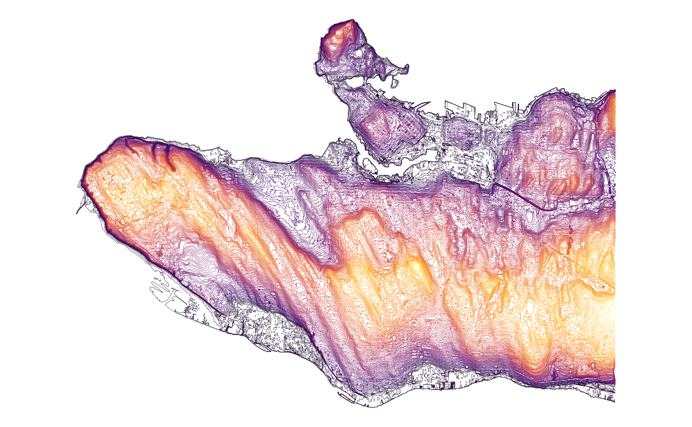
The same pattern works for any spatial dataset on the portal. Use
get_cov_metadata() to check whether a dataset has a
geo_shape field before downloading:
get_cov_metadata("elevation-contour-lines-1-metre-contours") |>
  dplyr::filter(type == "geo_shape")
#> # A tibble: 1 × 4
#>   name  type      label description
#>   <chr> <chr>     <chr> <chr>
#> 1 geom  geo_shape Geom  Spatial representation
To find spatial datasets in the first place, filter the catalogue on
the geo feature:
list_cov_datasets(refine = "features:geo") |>
  dplyr::select(dataset_id, title)
#> # A tibble: 135 × 2
#>    dataset_id                                       title
#>    <chr>                                            <chr>
#>  1 greenest-city-projects                           Greenest City projects
#>  2 olympic-transportation-plan-pedestrian-corridors Olympic transportation plan…
#>  3 lidar-2013                                       LiDAR 2013
#>  4 olympic-transportation-plan-venue-closure-areas  Olympic transportation plan…
#>  5 voting-places-2011                               Voting places 2011
#>  6 olympic-venues                                   Olympic venues
#>  7 greenways                                        Greenways
#>  8 wayfinding-map-stands                            Wayfinding map stands
#>  9 railways                                         Railways
#> 10 voting-places-2017                               Voting places 2017
#> # ℹ 125 more rows