Getting started: reading an older census table

This vignette walks through a typical use case: look up a table in the Statistics Canada catalogue, download and decode it, and work with the data.

This example uses an old table that is not available in any alternative format: the 1981 Census Profile for Canada, Provinces, Territories, Census Divisions and Census Subdivisions (97-570-X1981004). Modern census tables come with a tidy CSV and a Web Data Service API, and more recent vintages are also available in SDMX format, but the pre-2001 vintages are published only as Beyond 20/20 .ivt files — there is no CSV, no API, no easy-to-parse alternative. canivt decodes them straight from the bytes, so a 1981 profile becomes an ordinary data frame.

library(canivt)

(Optional) set a cache

canivt can cache downloaded .ivt files and the decoded Parquet so the second run is instant. Point it at a directory (e.g. in .Renviron via CANIVT_IVT_CACHE / CANIVT_DATA_CACHE, or per session):

options(
  canivt.ivt_cache  = "~/canivt-cache/ivt",   # raw .ivt downloads
  canivt.data_cache = "~/canivt-cache/data"   # decoded Parquet + catalogue
)

Without a cache everything still works; it just re-downloads each session. The IVT cache is not needed if the Parquet files are the primary target — omitting it reduces the storage footprint without impeding work with the cached Parquet files.

1. Look up the table in the catalogue

statcan_ivt_catalogue() scrapes the StatCan census datasets index into one tibble (one row per published table version), cached as Parquet after the first call. Each row carries the catalogue number, census_year, title, topic and the download URLs. The package ships with a cached version for convenience, but this can be replaced with an up-to-date scrape by passing the refresh = TRUE option.

catl <- statcan_ivt_catalogue()

# Find the 1981 census-division / subdivision profile
library(dplyr)
#> 
#> Attaching package: 'dplyr'
#> The following objects are masked from 'package:stats':
#> 
#>     filter, lag
#> The following objects are masked from 'package:base':
#> 
#>     intersect, setdiff, setequal, union
catl |>
  filter(census_year == 1981, grepl("Profile.*Census Divisions", title)) |>
  select(catalogue, census_year, title)
#> # A tibble: 2 × 3
#>   catalogue       census_year title                                             
#>   <chr>                 <int> <chr>                                             
#> 1 97-570-X1981004        1981 Census Profile for Canada, Provinces and Territor…
#> 2 97-570-X1981005        1981 Census Profile for Canada, Provinces and Territor…

If you already know the product id you can skip this step entirely and go straight to step 2.

2. Download and decode with get_statcan_ivt()

get_statcan_ivt() resolves the id against the catalogue, downloads the .ivt, decodes it, caches the result as Parquet, and hands back an arrow dataset connection. The second call skips the download and decode.

ds <- get_statcan_ivt("97-570-X1981004")
ds
#> FileSystemDataset with 1 Parquet file
#> 8 columns
#> geo_label: string
#> geo_name: string
#> geo_uid: string
#> values: string
#> profile: string
#> value: double
#> symbol: dictionary<values=string, indices=int8>
#> status: dictionary<values=string, indices=int8>
#> 
#> See $metadata for additional Schema metadata

The table is a classic profile: one row per geography × profile characteristic, with the count in value. The profile column holds the ~80 characteristics (population, age groups, mother tongue, tenure, …) and geo_name the bilingual place name.

ds |> distinct(profile) |> collect() |> head(6)

3. Query the data you want

Because ds is an Arrow dataset you can filter and select with dplyr verbs and only collect() the rows you need. Here we pull the mother-tongue counts (English / French / Other) for the ten provinces:

provinces <- c(
  "Newfoundland - Terre-Neuve", "Prince Edward Island - Île-du-Prince-Édouard",
  "Nova Scotia - Nouvelle-Écosse", "New Brunswick - Nouveau-Brunswick",
  "Quebec - Québec", "Ontario", "Manitoba", "Saskatchewan", "Alberta",
  "British Columbia - Colombie-Britannique"
)

res <- ds |>
  filter(
    geo_name %in% provinces,
    profile  %in% c("Mother tongue - English", "Mother tongue - French",
                    "Mother tongue - Other")
  ) |>
  select(geo_name, profile, value) |>
  collect()

That query returns 30 rows — the real decoded 1981 counts.

4. Work with the data

A little tidying — short province labels, and mother-tongue shares within each province — then a stacked bar chart. In 1981 Quebec is overwhelmingly French-mother-tongue while New Brunswick is the one clearly bilingual province:

library(ggplot2)

plot_data <- res |>
  mutate(province = sub(" - .*$", "", geo_name), # shorter province name
         mt = factor(sub("Mother tongue - ", "", profile),
                     levels = c("French", "Other", "English"))) |>
  mutate(share = value / sum(value), .by = province)

# order provinces by their French share
french_order <- plot_data |>
  filter(mt == "French") |>
  arrange(share) |>
  pull(province)

plot_data |>
  mutate(province = factor(province, levels = french_order)) |>
  ggplot(aes(share, province, fill = mt)) +
  geom_col(width = 0.75) +
  scale_x_continuous(labels = function(x) paste0(x * 100, "%"),
                     expand = expansion(mult = c(0, 0.03))) +
  scale_fill_manual(NULL,
    values = c(French = "#2c7fb8", Other = "#c7c7c7", English = "#d95f0e"),
    breaks = c("English", "French", "Other")) +
  labs(y = NULL, x = "Share of population",
       title = "Mother tongue by province, 1981 Census",
       caption = "Data: Decoded from the Beyond 20/20 .ivt file (97-570-X1981004)")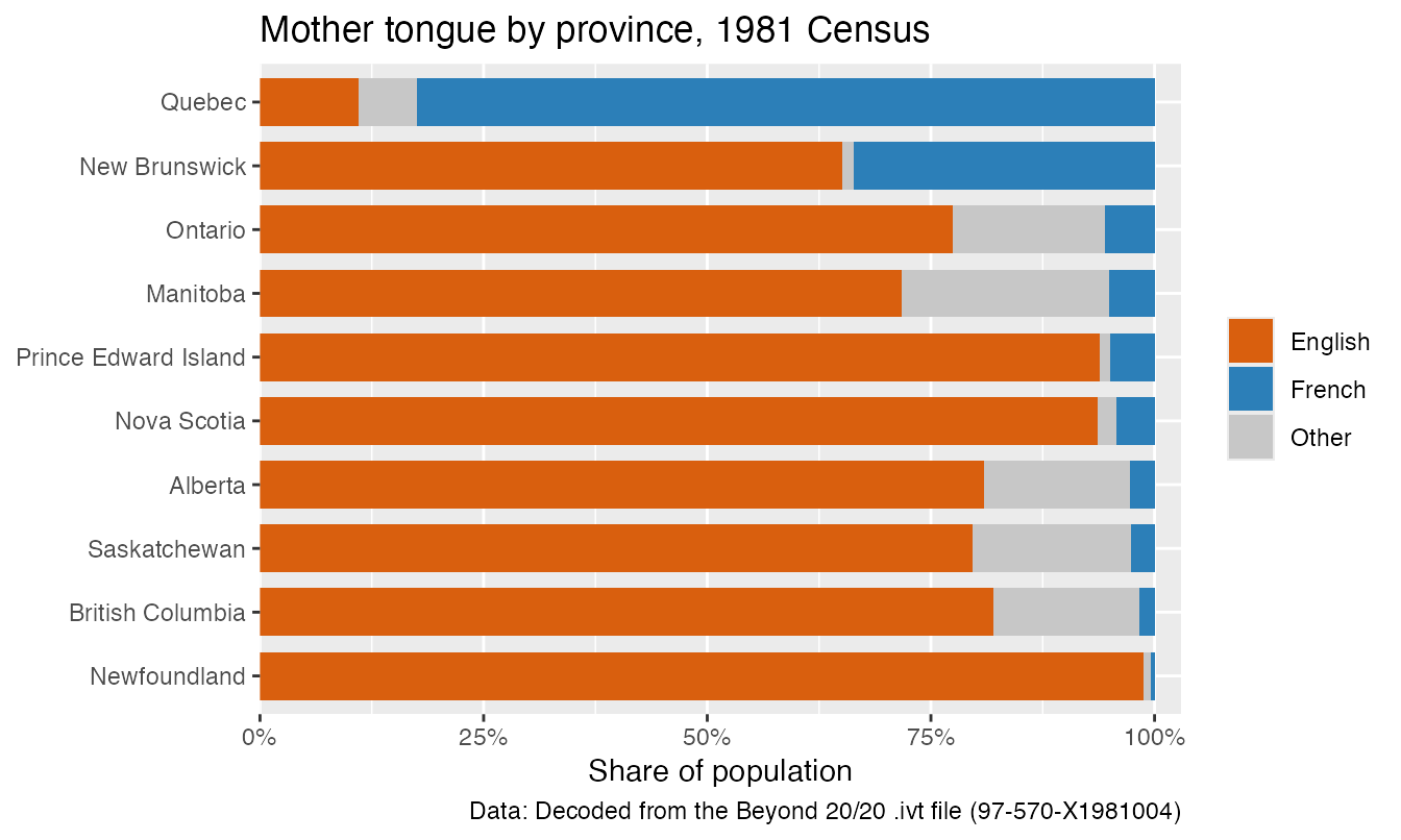

A note on cells that aren’t there

An IVT stores only the cells that have a value: zeros are not written, and neither are suppressed or not-applicable cells. What you get back, though, is the published table — every coordinate of the grid, exactly the rows StatCan’s own CSV download carries:

tab <- read_ivt("98100040.ivt")
ivt_tidy(tab)
#> ... value  symbol status
#>      24140  NA     NA               # a value
#>          0  NA     NA               # a published zero
#>         NA  x      Suppressed ...   # flagged, and why

Three kinds of row, and the difference between the last two is the point: completing the grid yourself from a stored-values-only table would turn every suppressed cell into a 0. The file does say which is which, in a status block after each page’s values, and that is what separates them here. Each flagged cell carries symbol and status in the file’s own words — the legend the table declares in its own header, so x means whatever this table says x means. attr(ivt_tidy(tab), "legend") is that legend.

read_ivt(complete = FALSE) gives you the raw store instead — smaller and faster, but then absence is ambiguous again, so pair it with missing = TRUE and ivt_missing() if you plan to fill the grid in. See ?read_ivt for the caveats: a page whose status block cannot be read has its absences published as zeros and warns rather than staying silent.

Recap

library(canivt); library(dplyr); library(ggplot2)

statcan_ivt_catalogue() |>                       # 1. find the table
  filter(census_year == 1981, grepl("Profile", title))

ds  <- get_statcan_ivt("97-570-X1981004")        # 2. download + decode + cache
res <- ds |> filter(...) |> collect()            # 3. query the slice you want
ggplot(res, ...) + geom_col()                    # 4. graph

The same four steps work for any table in the catalogue — 1981 profiles, 2021 dissemination-area crosstabs, commuting-flow tables — because read_ivt() (which get_statcan_ivt() calls) decodes every vintage through one path. For the full public API see ?read_ivt and ?get_statcan_ivt; for the binary format itself see vignette("ivt-format").