The Beyond 20/20 IVT file format

This vignette documents the Statistics Canada Beyond 20/20 .ivt binary format as reverse-engineered for canivt, and shows how the package’s functions map onto each part of the file. It is aimed at anyone who wants to understand, validate, or extend the parser. For day-to-day use see ?read_ivt. Two more detailed references ship with the package: the authoritative byte-format spec system.file("notes/ivt-format.md", package = "canivt"), and a terse catalog of every byte marker/signature the decoder keys on, system.file("notes/markers.md", package = "canivt") (self-checked by tests/testthat/test-markers.R).

One layout, one decoder

Every .ivt starts with a 4-byte signature ending 00 20 00; the modern census/custom lineage sets the leading byte to 04. (A second, older container generation sets it to 02 instead — see “An older survey-generation container” near the end of this vignette; everything in this section applies to both.) The file is one contiguous binary, and there is a single, descriptor-driven, name/type-agnostic decoder: it reads the dimension structure from the header, nests every dimension into a power-of-two positional bitmap (data dimensions innermost, geography outermost), and walks the value pages. What used to be documented as “family 1” and “family 2” are not two formats — they are two cases of this one layout, differing only in which dimension straddles the fixed 2048-bit (256-byte) page boundary:

• A data dimension straddles → geography is pushed fully into the page directory, one page per (geography, outer-data-coordinate). The reference table is 98-10-0241 (housing indicators by tenure; 166 geographies, 7 dimensions). Historically “family 1.”
• The data dimensions fit in ≤ 2048 bits → geography straddles: several geographies share each page’s presence record, and the directory is a flat list of geography-window pages. The reference table is 98-10-0023 (age × gender, down to dissemination areas; 63,404 geographies, 14.5 M cells). Historically “family 2.”

The 1991 census files (e.g. 1003011, E9101 — population by single year of age × sex) are the same container with pre-DGUID conventions: int16/int32 value pages and a bilingual, inline codebook. They decode through the same path.

read_ivt() auto-detects the case via ivt_family() (which just reports whether geography straddles), but the cell decode and metadata read are shared for every file — family only tags provenance. Every .ivt in the test corpus decodes, and no file in it is currently refused. That is not a promise about files the corpus has never seen: detection is structural, and read_ivt() still refuses anything whose page geometry it cannot verify rather than emit misindexed cells.

library(canivt)
tab <- read_ivt(ivt_download("98100023"))
tab
#> 
#> ── IVT table 98100023 ──────────────────────────────────────────────────────────
#> Age (in single years), average age and median age and gender: Canada, provinces
#> and territories, census divisions, census subdivisions and dissemination areas
#> 24347136 cells | 63404 geographies | 3 dimensions | 8 footnotes
#> geography labelled by uid (read_ivt(geo_attributes=TRUE) for names)
#> published grid: 23433112 values, 914024 flagged as missing

File layout at a glance

The high-level region order is the same for every IVT: a small header, the page directory, the value pages (which dominate — typically ~85–90 % of the file), then the codebook (geography identifiers/labels and the data dimension members), with footnotes near the tail. The bitmaps that make the format work all live inside the value pages, so they do not appear as regions at this scale — the next figure opens one page up.

library(ggplot2)
library(dplyr)

# Representative byte regions of the geography-straddle reference table
# 98-10-0023 (142,016,485 bytes), in file order. Every IVT follows this order.
regions <- data.frame(
  region = c("Header", "Page directory", "Value pages (data)",
             "Geography codebook", "Footnotes", "Dimension blocks (Age/Gender)"),
  size   = c(35950, 126800, 124122962, 17603000, 3000, 120485)
)

# Allocate a 20x10 = 200-tile waffle grid: each region gets tiles proportional
# to its byte size, but at least one tile so even the slivers show. The floor
# replaces the old ad-hoc per-region "exaggeration" scaling.
n_cols <- 20L
n_rows <- 10L
n_tiles <- n_cols * n_rows

alloc_tiles <- function(sizes, total, min_tiles = 1L) {
  tiles <- rep(min_tiles, length(sizes))     # everyone starts at the floor
  extra <- total - sum(tiles)                # tiles left to hand out
  ideal <- extra * sizes / sum(sizes)        # proportional, largest-remainder
  base  <- floor(ideal)
  tiles <- tiles + base
  short <- extra - sum(base)                 # rounding shortfall
  if (short > 0) {
    take <- order(ideal - base, decreasing = TRUE)[seq_len(short)]
    tiles[take] <- tiles[take] + 1L
  }
  tiles
}

regions$tiles <- alloc_tiles(regions$size, n_tiles)

# One row per tile, filled in file order, then wrapped onto the grid reading
# left-to-right, top-to-bottom.
regions$region <- factor(regions$region, levels = regions$region)
tile_region <- rep(regions$region, regions$tiles)
idx <- seq_along(tile_region) - 1L
tiles <- data.frame(
  region = tile_region,
  col    = idx %%  n_cols,
  row    = idx %/% n_cols
)

# legend label: real size plus the tile count it maps to
human <- function(b) ifelse(b >= 1e6, paste0(round(b / 1e6, 1), " MB"),
                     ifelse(b >= 1e3, paste0(round(b / 1e3),  " KB"),
                                      paste0(b, " B")))
labels <- paste0(regions$region, " — ", human(regions$size))

# One colourblind-safe categorical order (Okabe-Ito), shared with the page
# figure below so the two read as one system.
ivt_pal <- c("#0072B2", "#D55E00", "#009E73", "#E69F00", "#CC79A7", "#56B4E9")

ggplot(tiles, aes(x = col, y = row, fill = region)) +
  geom_tile(colour = "white", linewidth = 0.8, width = 0.95, height = 0.95) +
  scale_y_reverse(NULL, breaks = NULL, expand = c(0, 0)) +
  scale_x_continuous(NULL, breaks = NULL, expand = c(0, 0)) +
  scale_fill_manual(values = ivt_pal, name = NULL, labels = labels) +
  coord_equal() +
  labs(title = "IVT file layout — Table 98-10-0023 (142 MB)",
       subtitle = "One tile ≈ 0.5 % of the file; regions fill in file order (≥1 tile each)") +
  theme_minimal(base_size = 11) +
  theme(legend.position = "right", panel.grid = element_blank(),
        plot.title.position = "plot")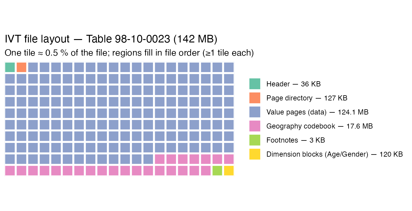

So roughly 87 % of the file is data; the geography codebook is the second-largest region (~12 %), and the header, directory, footnotes and per-dimension member blocks are slivers. All multi-byte integers are little-endian, and value runs frequently begin on odd (unaligned) byte offsets — a property that defeats naive aligned scans. Byte offsets in the parser are 0-based to match the layout.

Inside a value page: where the bitmaps are

A page is not just values. It has five regions in a fixed order, and three of them are bitmaps or bitmap-addressed:

[4-byte marker][presence bitmap][index bitmap][value run][cell-status tail]

The marker’s bytes give the widths of everything after it, so the whole page can be walked from its first four bytes. Two real pages, byte-exact:

# Measured directly from the page directory of two corpus tables:
# 98-10-0023 entry 1 (marker 88 01 20 08, float64, absent-mask tail) and
# 98-10-0128 entry 3 (marker a2 01 03 09, int16, status-array tail).
parts <- c("Page marker", "Presence bitmap", "Index bitmap",
           "Value run", "Cell-status tail")

page_parts <- data.frame(
  page  = rep(c("98-10-0023, entry 1\n3,296 B · mask tail",
                "98-10-0128, entry 3\n800 B · status array"), each = 5),
  part  = factor(rep(parts, 2), levels = parts),
  bytes = c(4, 256,  4, 2776, 256,
            4, 256, 34,  138, 368)
)

page_parts <- page_parts |>
  group_by(page) |>
  mutate(share = bytes / sum(bytes)) |>
  ungroup()

# The value run keeps the colour the waffle gives "Value pages (data)": this
# figure is a zoom into that region, so the region keeps its identity.
page_pal <- c("Page marker" = ivt_pal[1], "Presence bitmap" = ivt_pal[2],
              "Index bitmap" = ivt_pal[4], "Value run" = ivt_pal[3],
              "Cell-status tail" = ivt_pal[5])

# Label ink is chosen per fill, not per series, so the text stays legible.
ink <- c("Page marker" = "white", "Presence bitmap" = "white",
         "Index bitmap" = "grey15", "Value run" = "white",
         "Cell-status tail" = "white")

ggplot(page_parts, aes(x = share, y = page, fill = part)) +
  # reverse = TRUE lays the segments left-to-right in FILE order;
  # the 1.5pt surface gap keeps adjacent segments separable without a border hue
  geom_col(width = 0.55, colour = "white", linewidth = 1.5,
           position = position_stack(reverse = TRUE)) +
  geom_text(aes(label = ifelse(share > 0.07, paste0(bytes, " B"), ""),
                colour = part),
            position = position_stack(vjust = 0.5, reverse = TRUE),
            size = 3.1, fontface = "bold", show.legend = FALSE) +
  scale_x_continuous(NULL, expand = c(0, 0),
                     labels = function(x) paste0(x * 100, "%")) +
  scale_y_discrete(NULL, limits = rev) +
  scale_fill_manual(values = page_pal, name = NULL) +
  scale_colour_manual(values = ink, guide = "none") +
  labs(title = "Anatomy of one value page",
       subtitle = paste("Regions in file order, as a share of the page.",
                        "The 4-byte marker is too small to see here.")) +
  theme_minimal(base_size = 11) +
  theme(legend.position = "bottom", panel.grid = element_blank(),
        axis.text.y = element_text(hjust = 0, lineheight = 1.1),
        plot.title.position = "plot")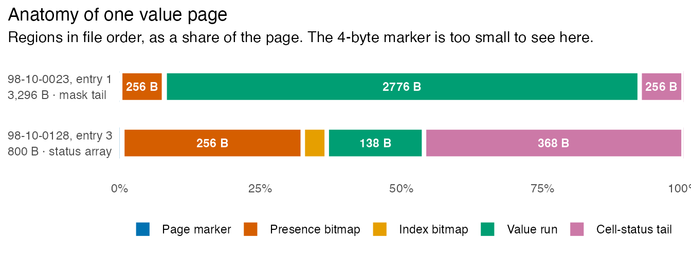

The two pages are the same structure with the weights redistributed. On the 98-10-0023 page the values dominate, as one would expect. On the 98-10-0128 page they do not: 138 bytes hold the 69 stored values while 402 bytes — half the page — describe what is absent, because that page’s grid is mostly “not applicable” and the file says so cell by cell.

The bitmap arrays, and what each one addresses

bitmap	where	one bit / word per	read as
Presence bitmap	every page, right after the marker	grid cell in the page — 1 = a value is stored	pair-swapped bytes, MSB-first
Index bitmap	every page, between presence and values (the marker’s trailer + head span)	width-byte word of the cell-status tail — 1 = that word was written	pair-swapped, MSB-first
Cell-status mask (0x8 pages)	the page tail, once the index is undone	grid cell — 1 = absent and a genuine zero	MSB-first, not pair-swapped
Cell-status codes (0xa pages)	the page tail, once the index is undone	grid cell, W bits each — a reason code, 0 = value or zero	MSB-first, not pair-swapped
Slot table	each dimension’s codebook block (81 02 <alloc> 16 00)	allocated member slot, 22 bits each — live / deleted, code length	pair-swapped, MSB-first
Footnote member bitmap	each dimension’s footnote region (84 01)	member — 1 = this member carries a note	member order

The presence and index bitmaps are read on every page of every read; the tail bitmaps only under read_ivt(complete = TRUE) (the default) or missing = TRUE. The two page-level bitmaps are nested, which is the part that is easy to miss: the index bitmap is a bitmap over a bitmap. The tail is stored sparsely — all-zero words are simply not written — so the index says which words are present, and the gate popcount(index) · width == tail length is what proves the page was read correctly. On the 98-10-0023 page above the index is 4 bytes = 32 bits, all set, addressing 32 float64 words = the 256-byte tail. On the 98-10-0128 page it is 34 bytes = 272 bits with 184 set, addressing 184 int16 words = the 368-byte tail; the other 88 words were all zero and never written.

Reading the layout from the header

The fixed header points at every major section, so the layout can be read up front without scanning for markers. ivt_f2_header_layout() (uniform across the modern and legacy formats) returns these as byte offsets:

header offset	section
u32 @32	dimension descriptor (per-dimension count, type, name + title)
u32 @40 / u32 @48	French / English title blocks — set in the legacy format, zero in the modern one (the version indicator)
u32 @552	geography field/attribute count (11 modern / 12 legacy)
u16 @558	page-directory start — low 16 bits only (the true start is u16 + k·65536 for the smallest k whose first entry validates; k = 0 for the reference tables, k > 0 for a few large tables)
u32 @572	codebook region start

A further section-pointer region (≈ @544..1080) is read the same way, each pointer resolving to a block directory of the identical 8-byte entry shape: @544 → the master directory (titles, the dimension descriptor, identity/notes blobs, product id), @712 → the data-quality-flag legend, and @824 + 14·(k−1) → the per-dimension codebook block directory (member labels, ordinals, footnotes) for dimension k. So the codebook, notes and legends are all located from the header, with bounded tail scans surviving only as fallbacks.

The page directory itself is a contiguous run of [u32 offset][u16 size][u16 size] records (the two sizes agree; the size is the page’s allocated length), in geography member order. Each record points at a page of value data.

Dimensions

The dimension descriptor declares each dimension uniformly. For 98-10-0023: Geography (63,404) × Age (128) × Gender (3). The decoder nests them positionally — geography outermost, the data dimensions inner in descriptor order with the last (here Gender) fastest-varying / the unit of value storage — and never asks which dimension is which by name or type byte. Geography is the first descriptor dimension in every layout except the profile lineage (a few 1981/1991 profile tables store a one-member “Values” placeholder first and put geography last); the nesting handles that with no special case, because it is purely positional. Exactly one dimension straddles the 2048-bit page boundary (§ below), which is what the historical “family” label really named.

meta <- ivt_metadata(ivt_download("98100023"))
data.frame(dimension = meta$dimension_names,
           members   = meta$dimension_counts)
#>                                           dimension members
#> 1                                         Geography   63404
#> 2 Age (in single years), average age and median age     128
#> 3                                            Gender       3

Three witnesses to the member count

Getting a dimension’s member count wrong misindexes every cell downstream, and the descriptor’s count field alone is not always trustworthy — its record framing is ambiguous in places, and a count can be read at the wrong width. The file states the same number three times, in three independent places, so the count is reconciled rather than taken on faith:

1. the descriptor record’s count field;
2. the codebook — the declared slot allocation and the length of the member arrays themselves. Member labels are written in blocks capped at 256, so a dimension with more members spans several blocks, and the run of block lengths witnesses the true total;
3. the page directory — how far the outermost paged dimension’s entries actually extend, counting only entries that both decode and carry cells.

Reconciliation only ever raises a count, never lowers one, and every correction is a loud, classed warning. When the count is right the container agrees exactly: the directory’s outer entry cartesian equals the page count.

Case A — geography straddles: a single page directory (98-10-0023)

When the data dimensions fit in one 2048-bit presence record, geography is the dimension that straddles the page boundary, so several geographies share each page and the directory is one flat list. Here each directory record is a page that packs 4 geographies:

[4-byte marker][4 × 64-byte presence records][index bitmap][dense value run][cell-status tail]

• the marker’s low nibble is the value width: 0x8 → float64, 0x4 → int32, 0x2 → int16 (so age counts are int16 but the average/median-age statistics are float64); its third byte encodes a trailer length and its fourth a head block of 32·(b3 − 8) bytes. Trailer and head together are not padding — they are the index bitmap described above, which is why the head grows exactly on the vintages that write a big cell-status tail;
• each geography’s presence is a 64-byte record stored byte-pair-swapped — swap adjacent bytes, then read a positional nibble per member, with the three genders Total/Men/Women at bits 3/2/1 (the all-present marker is 0xE);
• values are dense little-endian over the present (member, gender) cells, member-major / gender-inner. Only non-zero cells are stored — the StatCan CSV publishes the zeros, so an absent cell is either a zero or a missing value.

Which of the two it is is written down, in the page’s cell-status tail — see “Zeros, missing values, and the cell-status block” below, after the second straddle case.

The full per-geography codebook — name, DGUID, geographic level and type (+ abbreviation), two geocodes, the data-quality flag and note, and the non-response rate — decodes exactly for all 63,404 geographies; it is attached by read_ivt(geo_attributes = TRUE) (internally ivt_f2_geo_attributes()), while the default metadata path already carries the names and DGUIDs.

Case B — a data dimension straddles: per-geography directories (98-10-0241)

When the data dimensions alone overflow 2048 bits, a data dimension straddles instead and geography is pushed fully into the directory — each geography gets its own page directory at a fixed stride:

[0]            header: identity + dimension names
[37167]        geography index: one page-directory per geography, stride 0x1000
~1.08M..~55.4M value pages
~56.93M..EOF   footnote legend + codebook

Gotcha. The directories are grouped 8 to a 0x8000 region (288 entries used per 0x1000 slot, the rest zero-padded). Striding by 0x8000 instead of 0x1000 silently reads only every 8th geography — 21 of 166. The correct stride is 0x1000.

Here the page presence is a 256-byte positional, dimension-padded bitmap: 32-byte rows per Period; Statistics in 8-byte blocks; Housing indicators 0..5 within a block (the two bytes of each adjacent housing pair are byte-swapped, so housing h is read at stat*8 + bitwXor(h, 1)); and each presence byte’s bits 7..1 flag the 7 Tenure members (bit 0 padding). 0xFE therefore means “all 7 tenure values present”.

# bits 7..1 of 0xFE flag the 7 tenure members; bit 0 is padding
bitwAnd(bitwShiftR(0xFE, 7:1), 1L)
#> [1] 1 1 1 1 1 1 1
#> [1] 1 1 1 1 1 1 1

This is the same presence machinery as Case A, just with a data dimension in the straddle role: the presence granularity is the innermost dimension, the “all present” marker is 2^n − 2 over that bit width, the per-dimension strides are power-of-two padded and fixed, and one byte of each adjacent pair is swapped. The single decoder (ivt_layout() + ivt_decode()) computes the straddle dimension and these strides from the descriptor, so both cases run the identical code.

The padding itself is declared metadata, not a derived rule: every dimension’s codebook directory carries a member block (81 02 <alloc-u16> 16 00, or the survey generations’ time-series table ... 08 00) whose leading u16 is the dimension’s allocated member-slot capacity, and every nesting level — presence bits and directory strides alike — is padded to that allocation. It equals nextpow2(count) on almost every table, but not always: one Labour Force Historical Review table allocates 32 slots for a 10-member dimension, and its page directory faithfully spans the larger cartesian (the padding slots hold minimal, empty pages). Reading the declared allocation instead of re-deriving nextpow2 is what lets one layout rule cover that lineage too.

That block declares more than the capacity. Its mid-section is a table of 22 bits per allocated slot (pair-swapped, MSB-first): a live bit, the member code’s length in unary, and a flag for an extra trailing code byte. So the file states which slots hold members and which were deleted — the bitmap addresses members by slot, and slots can have holes. The declaration is trusted only when walking the code lengths it predicts consumes the following member-code array byte-exactly; where it does, the count and slot positions are read rather than guessed. The same slot map also addresses the codebook arrays, which may be written one record per allocated slot and left empty at the rest — an interior hole otherwise defeats a trailing-NA trim and silently shifts every label past it.

Zeros, missing values, and the cell-status block

Only non-zero cells are stored. The published table has zeros in it, so an absent cell is either a zero or a missing value — and the two are not the same number. Which one it is is written down in the file: every page can carry a cell-status block after its value run, and that block is what separates an absent-but-zero cell from an absent-and-missing one. So the familiar “absent means 0” shortcut is a simplification in every vintage, not just the modern ones; it merely looks true on tables that happen to publish no missing values.

Two forms, one storage rule

Which form a page uses is the marker’s high nibble.

• 0x8 — a bare one-bit-per-cell mask. It flags a subset of the absent cells, and that subset is the genuine zeros; the unflagged remainder is the missing data (the Beyond 20/20 viewer prints N). Where a table has no missing values the mask is exactly the complement of the presence bitmap, which is the common case and the reason it long looked redundant. Verified against the viewer on the 2001 census profile 97F0020XCB2001070.
• 0xa — a self-describing array of W-bit codes, one per cell, which says not just that a cell is missing but why. W is a storage choice, not a dialect — one file may mix widths — and code 0 always means a value or a genuine zero.

Both are stored the same way, and it is the storage rule that makes them one mechanism rather than two: a sparse array of value-width words, addressed by the page’s index bitmap, with all-zero words simply not written. The gate is the length identity popcount(index) · width == tail length, which holds on all 1,810,626 mask and 1,273,173 status-array pages of the development corpus. Rebuilding the block from that index is also what makes the 0xa array’s addressing general — it looked lineage-specific for years because each table’s dropped words shifted its codes by a different amount.

What the codes mean is declared by the file

The 0xa codes are numbered per table. A header slot holds the file’s own status legend — one record per code, with the symbol and its bilingual wording — and reading it is not optional, because the numbering is not universal: the modern NDM tables start at 1 = .., 2 = X, 3 = ..., while the 2016 98-400-X crosstabs and the older profiles start one symbol earlier, and the survey lineages have vocabularies of their own. Seven distinct legends appear across the corpus. Code 1 is each file’s own nothing here: filler at a padded grid position, the published symbol at a real cell — the grid decides which.

# the file's own legend, as read from its header
canivt:::ivt_f2_status_legend(readBin(path, "raw", file.size(path)))
#>    code symbol text_en
#> 1     1 ..     Not available for a specific reference period
#> 2     2 X      Suppressed to meet the confidentiality requirements …
#> 3     3 ...    Not applicable
#> 4     4 F      Too unreliable to be published
#> 5     5 0 s    value rounded to 0 (zero) where there is a meaningful …

Validated cell-exact against StatCan’s published tables on ten of them, in both directions — every published symbol matched by a code count and no code without a symbol — including 98-10-0128’s 1.86 M flagged cells.

This is what makes the published table possible

Both forms are decoded, and together they are what lets the package hand back the published table rather than the store:

x <- read_ivt(path)     # the published grid, the default
x$cells                 # every real coordinate: values, published zeros, and
                        # flagged cells as `value = NA` + `symbol` / `status`
attr(x$cells, "legend") # the file's own legend: code, symbol, EN and FR text

The completion rule is one sentence, and it is the block that licenses it: an absent cell is the published zero unless its page’s cell-status block says otherwise. Nothing in it comes from a published CSV — the grid is the layout’s, the exceptions are the tail’s — which is why it also applies to the tables that have no published CSV at all. Checked cell-for-cell against StatCan’s downloads on five tables covering every page class: every row present, none extra, no value differing, and every published symbol matched.

The two deviations are deliberate. A flagged cell gets value = NA where the CSV writes 0 beside the symbol, because a suppressed value is not a zero. And the symbol is reported verbatim from the file’s legend, so a table that stores X reports X even where the published legend prints x; mapping it would mean writing external ground truth into the parse path.

read_ivt(complete = FALSE) returns the store instead — smaller, and then the old caveat is back in force, so pair it with missing = TRUE. ivt_tidy_missing() labels those coordinates exactly as ivt_tidy() labels the values, and ivt_write_parquet() / ivt_write_csv() write them beside the data table as a _missing sidecar (ivt_missing() reads it back from any of these).

What is reported rather than hidden

Completeness is vintage-dependent, and every gap is counted rather than folded in: a file may use a code its own legend does not name, and a page whose index cannot reach the whole grid leaves the cells past it unclassifiable — published as zeros, and counted (canivt_absent_unclassified). (A mask that merely stops short is not one of those cases: all-zero words go unwritten, and since the index can address every word the grid spans on every corpus page, an unwritten one is the file stating that the cells it covers hold no zeros.) Each of those raises its own classed warning (canivt_status_unreadable, canivt_status_code_unknown, canivt_status_beyond_mask, …), so a missing count always comes with the caveats attached rather than hidden.

Whole-geography suppression is surfaced regardless, via metadata$geographies$has_data. See inst/notes/ivt-format.md for the byte layout, the legend’s own encoding, and the second (undecoded) tail block.

The codebook: labels, geographic ids, footnotes

The tail of the file holds the codebook: for each dimension, several parallel, member-ordered arrays of length-prefixed (“Pascal”: one length byte then that many text bytes) strings — member ordinals, the name (English then French) and, for Geography, the level, abbreviations, classification code, and full DGUID (2021A000011124 = Canada). Labels are encoded in Windows-1252: the 0x80–0x9F block carries real punctuation (e.g. 0x92 = the curly apostrophe in Tla'amin Lands), so the byte-class test that frames Pascal records must accept it — otherwise such a label aborts a record and splits the array mid-stream.

# labelled long table; read_ivt(geo_attributes = TRUE) attaches the full
# geography attribute table so tidy can label by name + level.
tab <- read_ivt(ivt_download("98100023"), geo_attributes = TRUE)
ivt_tidy(tab)
#> # A tibble: 24,347,136 × 9
#>    geo_label geo_name geo_uid        geo_level age   gender  value symbol status
#>    <chr>     <chr>    <chr>          <chr>     <chr> <chr>   <dbl> <fct>  <fct> 
#>  1 Canada    Canada   2021A000011124 Country   Tota… Total… 3.70e7 NA     NA    
#>  2 Canada    Canada   2021A000011124 Country   Tota… Men+   1.82e7 NA     NA    
#>  3 Canada    Canada   2021A000011124 Country   Tota… Women+ 1.88e7 NA     NA    
#>  4 Canada    Canada   2021A000011124 Country   0 to… Total… 6.01e6 NA     NA    
#>  5 Canada    Canada   2021A000011124 Country   0 to… Men+   3.09e6 NA     NA    
#>  6 Canada    Canada   2021A000011124 Country   0 to… Women+ 2.93e6 NA     NA    
#>  7 Canada    Canada   2021A000011124 Country   0 to… Total… 1.83e6 NA     NA    
#>  8 Canada    Canada   2021A000011124 Country   0 to… Men+   9.39e5 NA     NA    
#>  9 Canada    Canada   2021A000011124 Country   0 to… Women+ 8.92e5 NA     NA    
#> 10 Canada    Canada   2021A000011124 Country   Unde… Total… 3.43e5 NA     NA    
#> # ℹ 24,347,126 more rows

Footnotes are read from the header, not by scanning. Table-level (cube) notes come from the master directory; each dimension’s notes come from its per-dimension slot directory (the @824 + 14·(k−1) table above). Within a dimension each note carries a scope — a member note (annotating one geography or data member) or a whole-dimension note — resolved structurally: a 84 01 member bitmap opens the footnote region and lists, in member order, which members carry a note, so each note surfaces with its scope, owning dimension and member_id/member_refs. The text itself is tagged Footnote N (EN) / Renvoi N (FR); a bounded tail scan of those markers survives only as a loud fallback when the slot directories list none. (Those same Renvoi N texts also appear per-member in the geography directory’s tail as [01 01][u16 len-4][01] text blobs — told apart from member arrays by their NUL-free payload so they are not miscounted as attributes; see markers.md §F.) The legacy pre-DGUID files instead cite notes as (N) markers embedded in the member labels, linked back to the members that carry them.

str(meta$footnotes[[1]])
#> List of 7
#>  $ language   : chr "en"
#>  $ number     : int 1
#>  $ text       : chr "Age 'Age' refers to the age of a person (or subject) of interest at last birthday (or relative to a specified, "| __truncated__
#>  $ scope      : chr "dimension"
#>  $ dimension  : chr "Age (in single years), average age and median age"
#>  $ member_id  : int NA
#>  $ member_refs: int(0)
length(meta$footnotes)
#> [1] 8

The 1991 (pre-DGUID) files (1003011)

The 1991 census files are the same container in the geography-straddle case, with pre-DGUID conventions — fully decoded through the same read_ivt() path (cell-exact against the scraped Beyond 20/20 ground truth):

• value pages are int16/int32 (markers 0x82/0x84) rather than float64, and presence uses the same byte-pair-swapped positional bitmap;
• geography is a single inline block per chunk of "<name> (<GEOUID>) <flag>" — a bilingual name (Newfoundland | Terre-Neuve), a bare GEOUID (a shortened DGUID without the year/area-type prefix), and a data-quality flag;
• the table identity is stored out of line (the @40/@48 header pointers, which are zero on the modern DGUID files — that difference is the format-version signal), and footnotes are the (N) text form described above.

A profile lineage of pre-DGUID files (some 1981/1991 profiles) additionally puts geography last behind a one-member “Values” placeholder; the positional nesting absorbs that without a special case.

Pre-2016 tables predate the modern 8-digit b2020 .zip endpoint that ivt_download() uses, so fetch the raw .ivt through its catalogue row (statcan_ivt_download() resolves the Download.cfm?PID= link and returns the local path), then read it the same way:

row <- subset(statcan_ivt_catalogue(), catalogue == "1003011")
leg <- read_ivt(statcan_ivt_download(row))   # 41,859 geographies, Age(110) × Sex(3)
ivt_tidy(leg)
#> # A tibble: 13,813,470 × 8
#>    geo_label geo_name geo_uid single             sex         value symbol status
#>    <chr>     <chr>    <chr>   <chr>              <chr>       <dbl> <fct>  <fct> 
#>  1 Canada    Canada   00      Total - Age Groups Total - S… 2.73e7 NA     NA    
#>  2 Canada    Canada   00      Total - Age Groups Male       1.35e7 NA     NA    
#>  3 Canada    Canada   00      Total - Age Groups Female     1.38e7 NA     NA    
#>  4 Canada    Canada   00      0-4 years          Total - S… 1.91e6 NA     NA    
#>  5 Canada    Canada   00      0-4 years          Male       9.76e5 NA     NA    
#>  6 Canada    Canada   00      0-4 years          Female     9.31e5 NA     NA    
#>  7 Canada    Canada   00      Under 1            Total - S… 3.94e5 NA     NA    
#>  8 Canada    Canada   00      Under 1            Male       2.02e5 NA     NA    
#>  9 Canada    Canada   00      Under 1            Female     1.92e5 NA     NA    
#> 10 Canada    Canada   00      1                  Total - S… 3.95e5 NA     NA    
#> # ℹ 13,813,460 more rows

An older survey-generation container (02 00 20 00)

A second, older Beyond 20/20 container generation shares the same page/value/ codebook model but starts with 02 00 20 00 instead of 04 00 20 00 — byte 0 is a container-generation tag, not part of a fixed constant, and ivt_family()/read_ivt() handle both transparently. This generation covers older survey product lines rather than census geography tables: Health Statistics at a Glance (1999), the 1996 Census of Agriculture, the 1996 Small Area Business survey, and the provincial Canadian Business Patterns releases of 1997–2002 (see “Undeclared geometry” below).

Two things are structurally different, both confined to the descriptor and codebook:

• No geography dimension. These are single-area survey products — the REGION/GEOGRAPHY dimension carries no DGUID or geographic identifiers, so read_ivt() treats it as an ordinary, fully-labelled data dimension: metadata$geographies is empty and cells has no geo column.
• Generated time-series labels. A reference/time dimension can be stored with no code or label array at all — only a per-member date table (one-byte populated-slot flags + a 3-byte date, days since 0000-03-01). Member labels (typically a year) are generated from those dates. The slot addressing is the same one described above — this table (... 08 00) is simply where a dimension declares it when it carries no 16 00 member-code block. A dimension carries one or the other, never both.

# Health Statistics at a Glance 1999 is Borealis-hosted (see vignette("borealis")
# for browsing/downloading): Quantifier x Geography x Period, no geography
# dimension, year labels generated from the on-disk dates.
path <- borealis_ivt_download(hits[1, ])   # hits from borealis_ivt_catalogue()
hsg  <- read_ivt(path)
ivt_tidy(hsg)

Values in this generation are complete integers in the indicator’s own unit — not a fixed-point encoding needing a decimal scale. The unit is stated in the relevant member’s description text, surfaced via ivt_members()’s description/description_fr columns where it can be mapped unambiguously.

See inst/notes/ivt-format.md (“The older 02 00 20 00 survey-generation container”) and inst/notes/markers.md §E.1 for the exact byte framings.

Undeclared geometry: the provincial Business Patterns cluster

One corner of this generation declares less than everything above assumes. The provincial Canadian Business Patterns releases (PROVSIC*, PRVNAIC*, CACMA*, 1997–2002; province/CMA × industry × employment-size class) carry no 16 00 slot table for any dimension, so the outer directory stride — the number of entry slots each geography occupies — is stated nowhere in the file and has to be measured from the page directory itself. It is measured as a tiling, not a progression: every geography occupies S consecutive entry slots and writes the same window residues inside them, and the smallest S that tiles the whole directory wins. That matters because a run need not start at window 0 — one file lays its 11 industry windows at slots 3..13 of a 16-slot group. A written page whose presence record is entirely zero is treated as an absence: it carries no cells, so it witnesses nothing about where members sit.

Because the geometry is inferred rather than declared, it is adopted only if the decoded values reconcile exactly on the file’s own arithmetic — the industry Total member equalling the sum of the detail members for every (geography, size class), or Canada equalling the sum of the provinces. A file whose geometry cannot be measured, or whose decode does not reconcile, is left unsupported rather than emitting unvalidated numbers.

Two caveats travel with these tables, both raised as loud, classed warnings:

• the industry labels are provisional (canivt_suba_labels) — reconciliation validates the sums, not the code → member assignment, and a uniform relabel would leave every sum unchanged. There is no published ground truth to settle it against;
• the recovered geometry itself is flagged (canivt_suba), so a caller can spot these tables programmatically or promote the warnings to errors with options(canivt.strict = TRUE).

Values and dimension structure are otherwise ordinary. See R/suba.R and the sub-A sections of inst/notes/unsupported-formats.md and inst/notes/coverage.md.

How canivt maps to the format

Region	Function(s)	Source file(s)
Header identity, dimension descriptor, layout	ivt_metadata(); (internal) ivt_f2_header_layout(), ivt_f2_descriptor()	R/codebook-f2.R, R/dimdir.R
Page directory / geography index	(internal) ivt_layout()	R/decode.R, R/container*.R
Presence bitmap + value codec (both straddle cases)	(internal) ivt_decode()	R/decode.R, R/decode-f2.R
Index bitmap + cell-status tail (zeros vs missing)	read_ivt(missing = TRUE), ivt_missing(), ivt_tidy_missing(); (internal) ivt_page_status(), ivt_f2_status_legend()	R/status.R, R/complete.R
Codebook labels, DGUIDs/GEOUIDs, geography attributes, footnotes	ivt_metadata(), read_ivt(geo_attributes = TRUE); (internal) ivt_f2_geo_attributes()	R/codebook-f2.R, R/dimdir.R, R/read-f2.R
Tidy / write outputs	ivt_tidy(), ivt_write_*()	R/read.R, R/write.R

Validation

canivt is validated against the StatCan CSV/metadata downloads: the data-dimension-straddle reference (98-10-0241) all 166 geographies and 7,489,464 cells exact; the geography-straddle reference (98-10-0023) all 63,404 geographies and 14.5 M cells exact, plus every geography attribute and the Age/Gender labels; and the 1991 table (1003011) cell-exact for all scraped ground-truth geographies. The unified decoder is additionally byte-identical to the two former decoders on six reference tables, and viewer/CSV-validated across the wider corpus — 1996–2021 census tables, 1981/1991 profiles, 2001/2006 F-series, large 2016 98-400-X crosstabs, commuting-flow tables, custom extracts, the Business Register lineage, and the older 02 00 20 00 survey generation. The published table — the completion of the store with its zeros and flagged cells — is validated separately, cell-for-cell against StatCan’s own CSVs on five tables covering every page class, and corroborated by the WDS nbDatapointsCube count equalling stored + flagged.

Three opt-in regression ledgers run the whole local corpus through read_ivt(): the stored cell count per table, the cell-status tail per table (unreadable and contradictory must stay at zero), and the fold (stored + zeros + flagged == rows == grid). For older vintages the package scrapes the Beyond 20/20 web viewer for ground-truth data to validate against. See the tests/ directory and the notes file (inst/notes/coverage.md, decode-history.md) for the exact figures.