Unabsorbed Stock

Jens von Bergmann

2017-09-22

CMHC data

library(dplyr)
library(tidyr)
library(ggplot2)
#devtools::install_github("mountainmath/cmhc")
library(cmhc)

cma="Vancouver"
year=2017
month=12
breakdown_geography_type='CT'

table_id=paste0(cmhc_table_list["Scss Unabsorbed Inventory Base"], ".9")


census_cma=census_geography_list[[cma]]
cma_header=substr(census_cma, nchar(census_cma)-2,nchar(census_cma))

#get all under construction data for Vancouver and pad CT GeoUIDs.
unabsorbed <- get_cmhc(cmhc_snapshot_params(
  geography_id = cmhc_geography_list[[cma]],
  breakdown_geography_type = breakdown_geography_type,
  table_id=table_id,
  year = year,
  month = month)) %>%
  rename(GeoUID = X1) 

if (breakdown_geography_type=="CT") {
  census_cma=census_geography_list[[cma]]
  cma_header=substr(census_cma, nchar(census_cma)-2,nchar(census_cma))
  unabsorbed <- unabsorbed %>%  mutate(GeoUID = cmhc_geo_uid_for_ct(cma_header,GeoUID)) 
}

Geographic data

library(cancensus)
library(ggplot2)
library(sf)
library(RColorBrewer)
#options(cancensus.api_key='your API key')
geos <- get_census(dataset = 'CA16', regions=list(CMA=census_cma),level=breakdown_geography_type,geo_format='sf')

Joining the data

if (breakdown_geography_type=='CT') {
geos <- left_join(geos,unabsorbed, by=c("GeoUID"="GeoUID"))
} else {
geos <- left_join(geos,unabsorbed, by=c("name"="GeoUID"))
}

Graph

bg_color="#eeeeee"
theme_opts<-list(theme(panel.grid.minor = element_blank(),
                       #panel.grid.major = element_blank(), #bug, not working
                       panel.grid.major = element_line(colour = bg_color),
                       panel.background = element_rect(fill = bg_color, colour = NA),
                       plot.background = element_rect(fill=bg_color, size=1,linetype="solid"),
                       axis.line = element_blank(),
                       axis.text.x = element_blank(),
                       axis.text.y = element_blank(),
                       axis.ticks = element_blank(),
                       axis.title.x = element_blank(),
                       axis.title.y = element_blank()))

After defining a basic theme we can go ahead and map the data.

type="Apartment"

geos[[type]][geos[[type]]==0] <- NA

ggplot(geos) +
  geom_sf(aes_string(fill = type), size = 0.05) +
  scale_fill_viridis_c("Units", option="inferno") +
  ggtitle(paste0(cma, " CMA Unabsorbed ",type," Units ",month,"-",year," (",prettyNum(sum(geos[[type]],na.rm=TRUE),big.mark = ",")," total)")) +
  theme_opts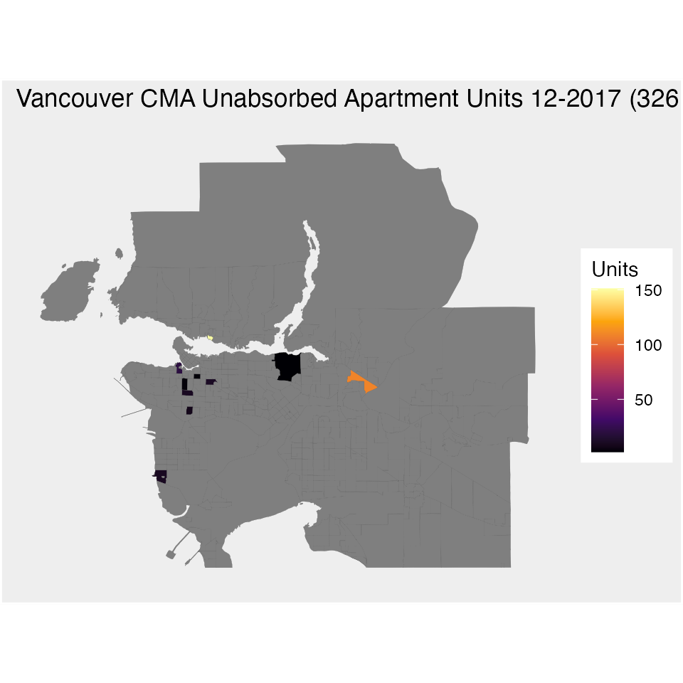

type="Row"

geos[[type]][geos[[type]]==0] <- NA

ggplot(geos) +
  geom_sf(aes_string(fill = type), size = 0.05) +
  scale_fill_viridis_c("Units", option = "magma") +
  ggtitle(paste0(cma, " CMA Unabsorbed ",type," Units ",month,"-",year," (",prettyNum(sum(geos[[type]],na.rm=TRUE),big.mark = ",")," total)")) +
  theme_opts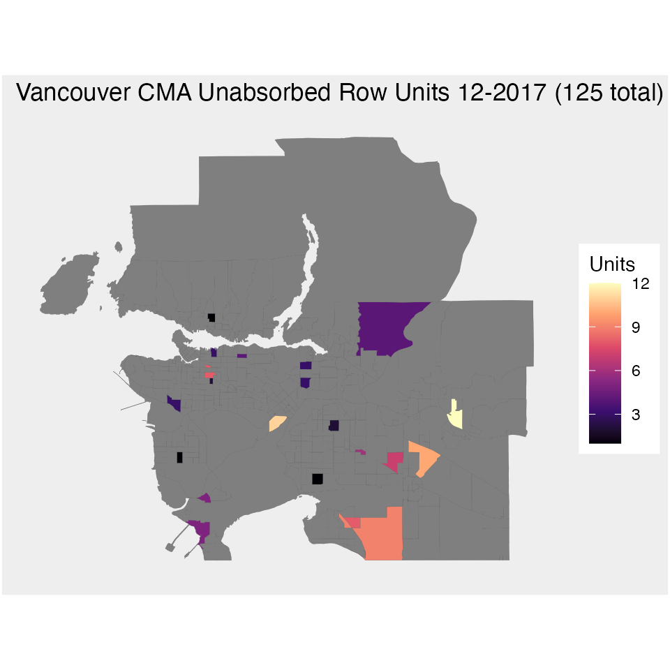

type="All"

geos[[type]][geos[[type]]==0] <- NA

geos$units=cut(geos$All,breaks=c(0,1,5,10,50,100,200))

ggplot(geos) +
  geom_sf(aes_string(fill = "units"), size = 0.05) +
  scale_fill_viridis_d("Units", option = "magma",na.value="grey") +
  ggtitle(paste0(cma, " CMA Unabsorbed ",type," Units ",month,"-",year," (",prettyNum(sum(geos[[type]],na.rm=TRUE),big.mark = ",")," total)")) +
  theme_opts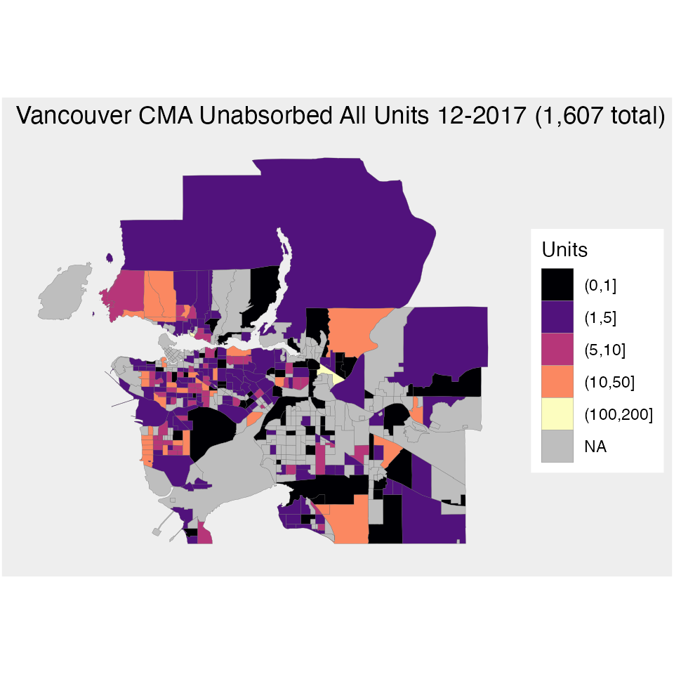

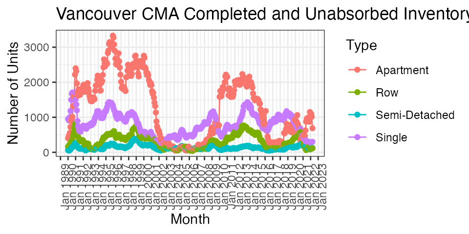
table="Scss Unabsorbed Inventory Time Series"
level="CMA"
cmhc_params=cmhc_timeseries_params(table_id = cmhc_table_list[table], region = cmhc_region_params(cma,level))               
data <- get_cmhc(cmhc_params)  %>% rename(Date=X1) %>% mutate(Date= as.Date(paste0("01 ",Date),format="%d %b %Y"))
types <- names(data)[!names(data) %in% c("Date")]
#data[is.na(data)] <- 0

plot_data=data %>% pivot_longer(all_of(types),names_to="Type",values_to="Units") 

ggplot(plot_data %>% filter(Type %in% c("Row","Apartment","Single","Semi-Detached")),aes(x=Date, y=Units, color=Type, group=Type)) +
  geom_path() +
  geom_point() +
  scale_x_date(date_breaks = "1 year",date_labels = "%b %Y") +
  theme_bw() + 
  labs(y="Number of Units",
       x="Month",
       title=paste0(cma," ",level," Completed and Unabsorbed Inventory")) +
  theme(axis.text.x = element_text(angle = 90, hjust = 1))