Rental Under Construction

This vignette demonstrates how to pull in under construction data from CMHC using the cmhc package, link it with geographic data from CensusMapper using the cancensus package and map the under construction data. ## CMHC data

library(dplyr)
#devtools::install_github("mountainmath/cmhc")
library(cmhc)

cma="Vancouver"
year=2017
month=10
breakdown_geography_type='CSD'

table_id=cmhc_table_list[paste0("Scss Under Construction", " ", breakdown_geography_type)]


census_cma=census_geography_list[[cma]]
cma_header=substr(census_cma, nchar(census_cma)-2,nchar(census_cma))

#get all under construction data for Vancouver and pad CT GeoUIDs.
rental_under_construction <- get_cmhc(cmhc_snapshot_params(
  geography_id = cmhc_geography_list[[cma]],
  breakdown_geography_type = breakdown_geography_type,
  filter=list("dimension-18"="Rental"),
  table_id=table_id,
  year = year,
  month = month))
rental_under_construction <- rental_under_construction %>%
  rename(GeoUID = X1) 
all_under_construction <- get_cmhc(cmhc_snapshot_params(
  geography_id = cmhc_geography_list[[cma]],
  breakdown_geography_type = breakdown_geography_type,
  table_id=table_id,
  filter=list("dimension-18"="All"),
  year = year,
  month = month))
all_under_construction <- all_under_construction %>%
  rename(GeoUID = X1)

uc=inner_join(all_under_construction,rental_under_construction,by="GeoUID") %>%
  mutate(rental_pct=All.y/All.x)
total=sum(uc$All.x)
rental=sum(uc$All.y)

if (breakdown_geography_type=="CT") {
  census_cma=census_geography_list[[cma]]
  cma_header=substr(census_cma, nchar(census_cma)-2,nchar(census_cma))
  uc <- uc %>%  mutate(GeoUID = cmhc_geo_uid_for_ct(cma_header,GeoUID)) 
}

Geographic data

library(cancensus)
library(ggplot2)
library(sf)
library(RColorBrewer)
#options(cancensus.api_key='your API key')
geos <- get_census(dataset = 'CA16', regions=list(CMA=census_cma),level=breakdown_geography_type,geo_format='sf')

Joining the data

if (breakdown_geography_type=='CT') {
geos <- left_join(geos,uc, by=c("GeoUID"="GeoUID"))
} else {
geos <- left_join(geos,uc, by=c("name"="GeoUID"))
}

Graph

bg_color="#c0c0c0"
theme_opts<-list(theme(panel.grid.minor = element_blank(),
                       #panel.grid.major = element_blank(), #bug, not working
                       panel.grid.major = element_line(colour = bg_color),
                       panel.background = element_rect(fill = bg_color, colour = NA),
                       plot.background = element_rect(fill=bg_color, size=1,linetype="solid"),
                       axis.line = element_blank(),
                       axis.text.x = element_blank(),
                       axis.text.y = element_blank(),
                       axis.ticks = element_blank(),
                       axis.title.x = element_blank(),
                       axis.title.y = element_blank()))

After defining a basic theme we can go ahead and map the data.

ggplot(geos) +
  geom_sf(aes(fill = rental_pct), size = 0.05) +
  scale_fill_viridis_c("%RENTAL") +
  ggtitle(paste0(cma, " CMA Under Construction ",month,"-",year," (",prettyNum(total,big.mark = ",")," total, ",prettyNum(rental,big.mark = ",")," rental)")) +
  theme_opts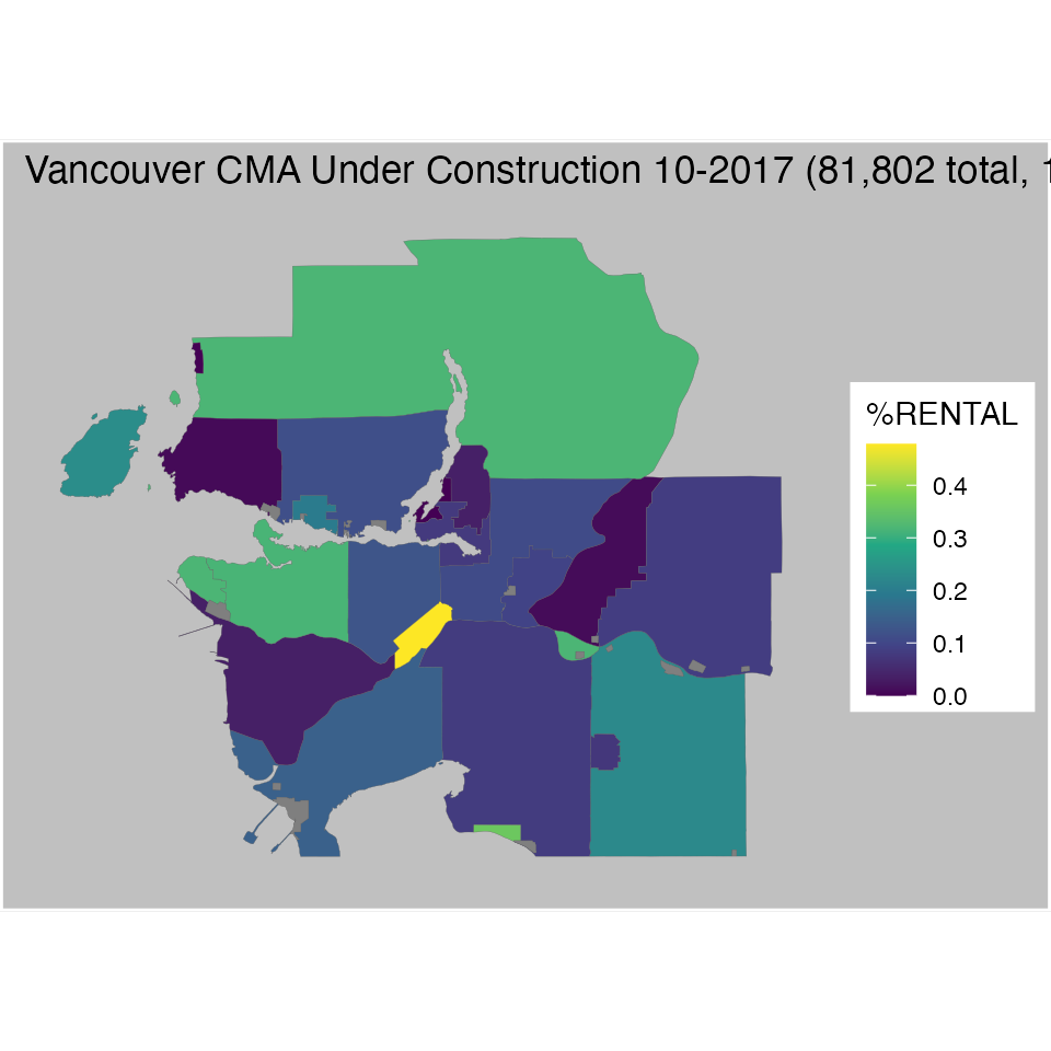

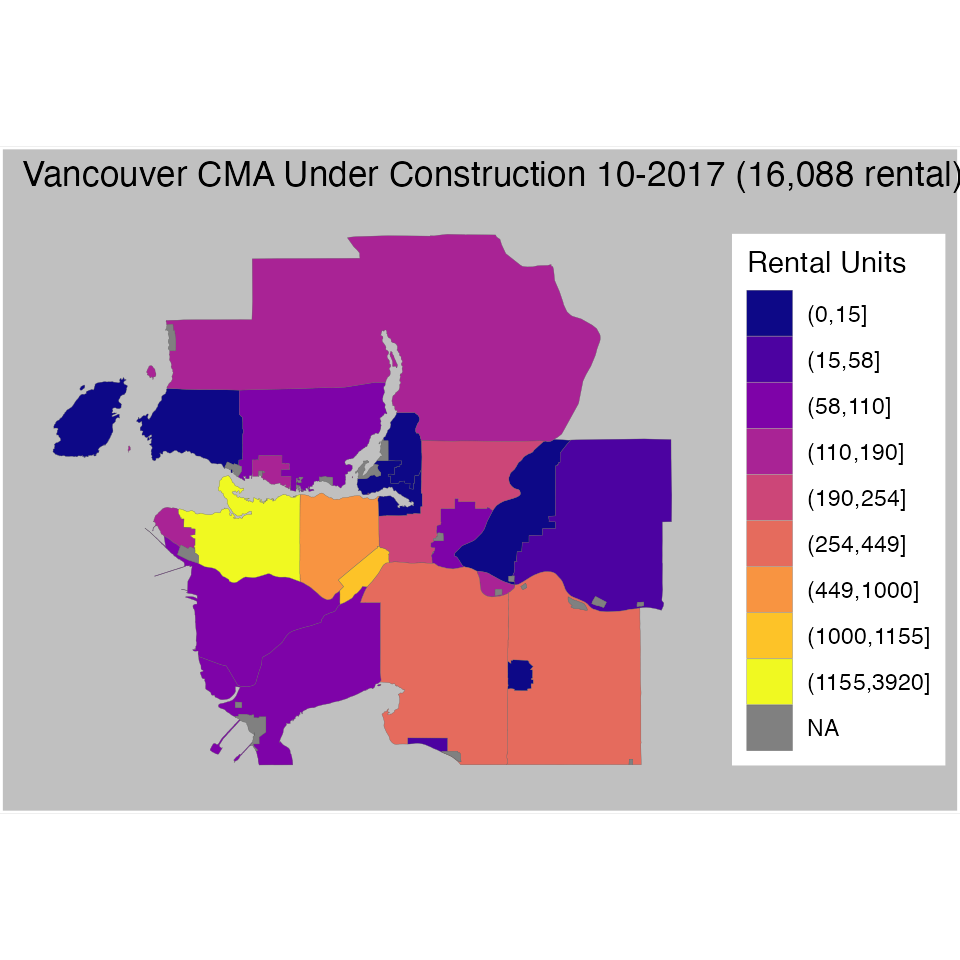
library(classInt)
breaks=classIntervals(geos$All.y, n = 9, style = "jenks")
geos <- geos %>% mutate(`Rental Units` = cut(geos$All.y, breaks = c(breaks$brks), dig.lab = 4))
ggplot(geos ) +
  geom_sf(aes(fill = `Rental Units`), size = 0.05) +
  scale_fill_viridis_d("Rental Units",option = "plasma",na.value='#808080') +
  ggtitle(paste0(cma, " CMA Under Construction ",month,"-",year," (",prettyNum(rental,big.mark = ",")," rental)")) +
  theme_opts

Jens von Bergmann

2017-09-22

Geographic data

Joining the data

Graph