13 Land and building values
The Globe and Mail reported that
“between 2006 and 2022, Vancouver building values stayed the same while the land value increased by more than 500 per cent”.
To anyone familiar with Vancouver during this time frame the claim that “building values stayed the same” seems questionable. This brings us to our question.
13.1 Question
How have land and building values in Vancouver changed since 2005 (2006 tax assessment year)?
13.2 Data sources
Land and building values are assessed separately by BC Assessment, and we will piggy-back of their estimates instead of trying to estimate them ourselves. The City of Vancouver makes assessment data for the City available on their Open Data Portal.
13.3 Data acquisition
The VanouvR package (“VancouvR: Access the ’City of Vancouver’ Open Data API” 2019) makes it easy to access this data in R and one of the package vignettes has code that does pretty much what we need.
The datasets in question are the property-tax-report, due to size the data is split over several datasets.
Code
search_cov_datasets("property-tax-report") |>
  select(dataset_id,title)
# A tibble: 4 × 2
dataset_id title
<chr> <chr>
1 property-tax-report-2016-2019 Property tax report 2016-2019
2 property-tax-report-2011-2015 Property tax report 2011-2015
3 property-tax-report Property tax report
4 property-tax-report-2006-2010 Property tax report 2006-2010The first tax assessment year in the dataset is for 2006, the last one is for the current year, 2024 as of the writing of this. Assessments are pegged to July 1st of the previous year, so we have data for all years from July 2005 through 2023. This is likely the same data source that news article used, except that the article did not adjust to the date the assessments are pegged to.
For our purposes all we need is aggregates for each year, the Open Data Portal allows server side aggregation of data and the R package supports that. This cuts down on time and the amount of data we need to transfer. We simply group by tax assessment year and aggregate up the assessed land and building values for each year.
Code
land_building_data_raw <-search_cov_datasets("property-tax-report") |>
    pull(dataset_id) |>
    map_df(function(ds) aggregate_cov_data(
      ds,
      group_by="tax_assessment_year as Year",
      select="sum(current_land_value) as Land, sum(current_improvement_value) as Building")) |>
  arrange(Year)
This gives us a simple data frame with land and building values for each year. We check on the tax years in question, as well as the most recent one.
13.4 Data preparation
There is not much to do here, we remember that assessments are pegged to July 1st in the previous year and reshape the data into long form.
Code
land_building_data <- land_building_data_raw |>
    mutate(Date=as.Date(paste0(as.integer(Year)-1,"-07-01"))) |>
    pivot_longer(c("Land","Building"),names_to = "Component")
13.5 Analysis and visualization
Let’s take a quick look what that data looks like.
Code
ggplot(land_building_data,aes(x=Date,y=value,colour=Component)) +
  geom_line() +
  scale_y_continuous(labels=\(x)scales::dollar(x,scale=10^-9,suffix="bn")) +
  expand_limits(y=0) +
  labs(title="City of Vancouver assessed land and building values",
       y="Assessed value",
       x=NULL,
       caption="CoV Open Data")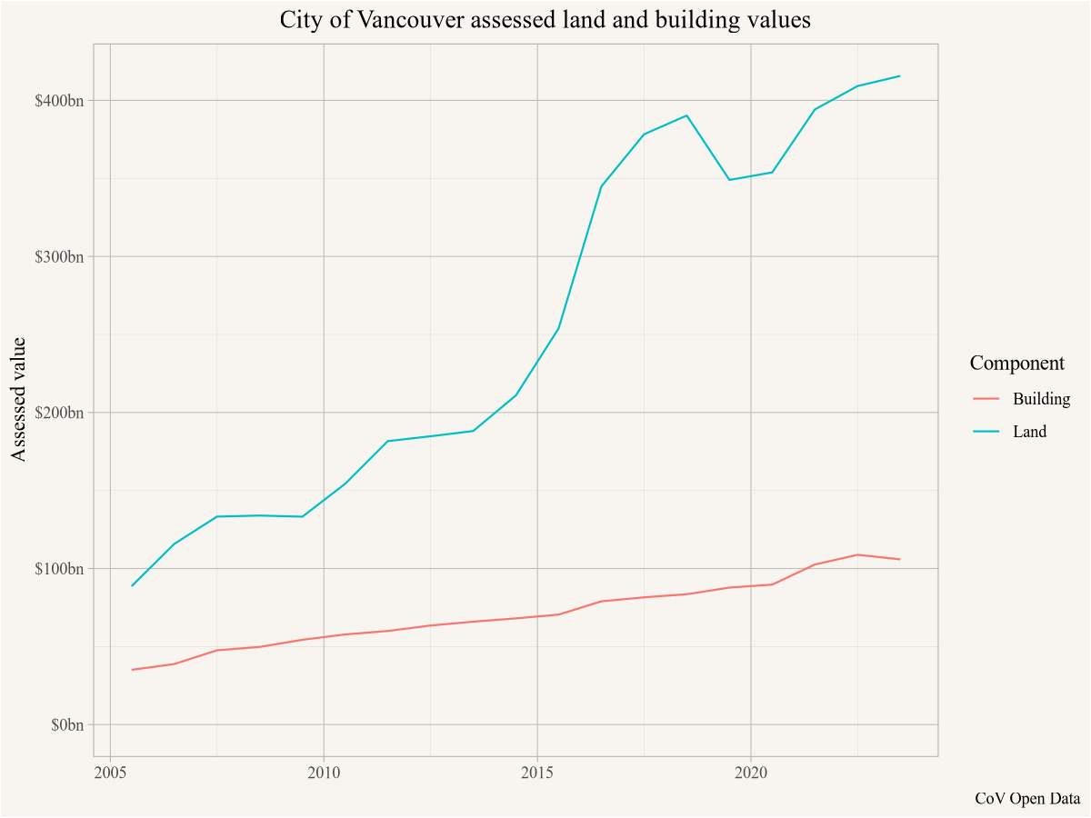
So far so good, but we should probably account for inflation. We borrow code from the section on income change to pull CPI data and fold it in.
Code
library(cansim)
inflation <- get_cansim_vector("v41693271") |>
  mutate(Date=Date %m+% months(6)) |>
  select(Date,CPI=val_norm) |>
  filter(Date %in% land_building_data$Date) |>
  mutate(CPI=CPI/last(CPI,order_by = Date))

land_building_data |>
  left_join(inflation,by="Date") |>
ggplot(aes(x=Date,y=value/CPI,colour=Component)) +
  geom_line() +
  scale_y_continuous(labels=\(x)scales::dollar(x,scale=10^-9,suffix="bn")) +
  expand_limits(y=0) +
  labs(title="City of Vancouver assessed land and building values",
       y="Assessed value (July 2023 dollars)",
       x=NULL,
       caption="CoV Open Data")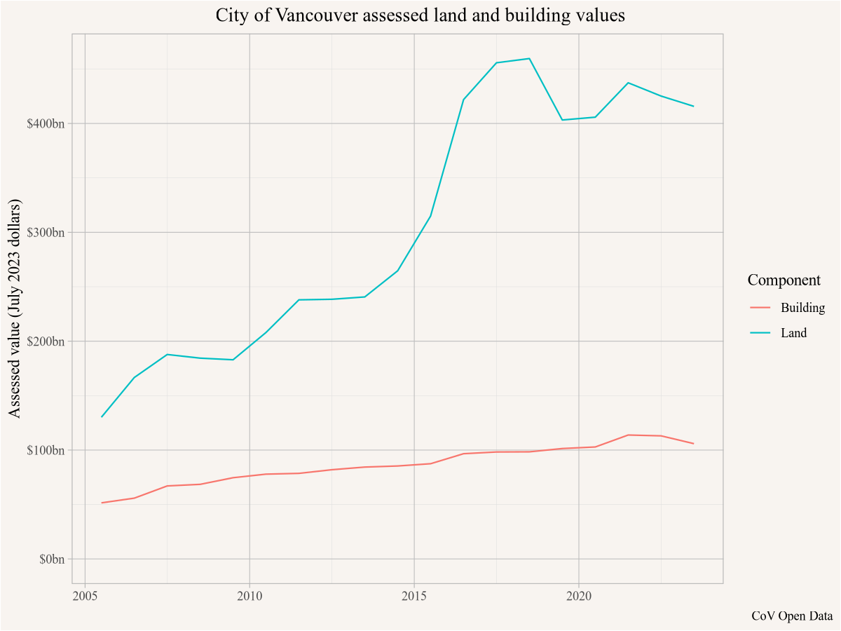
As we might have expected, values rose faster than inflation, but they did so for buildings as well as for land. The land value change is impressive, but it’s hard to judge that against the building value change, which started at a much lower value. The article looked at percentage change, so let’s do the same.
Code
plot_data <- land_building_data |>
  left_join(inflation,by="Date") |>
  mutate(real_value=value/CPI) |>
  mutate(real_ratio = real_value/first(real_value,order_by=Date),
         ratio = value/first(value,order_by=Date),
         .by=Component)

ggplot(plot_data,aes(x=Date,y=real_ratio,colour=Component)) +
  geom_line() +
  scale_y_continuous(labels=\(x)scales::percent(x-1),
                     trans="log",breaks=seq(1,5)) +
  labs(title="City of Vancouver assessed land and building values",
       y="Real change since July 1, 2005",
       x=NULL,
       caption="CoV Open Data")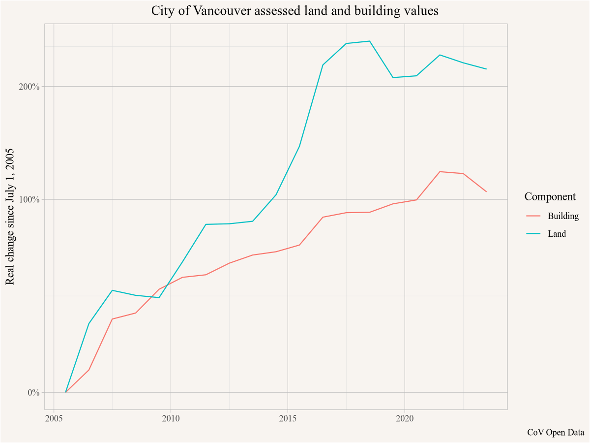
Since this is ratio data we chose a logarithmic scale on the y-axis. This shows that between 2005 and 2021 (so using assessment years 2006 and 2022) real land values increased by 236% and building values by 121% . Maybe the article was using nominal value increases, in nominal terms land increased by 345% and building values by 192%.
13.6 Interpretation
The increase in land values is lower than the “more than 500 per cent” claimed in the article, and the claim that “building values stayed the same” is clearly false.
What is clear is that land values have risen faster than building values, likely in large part because restrictive zoning has prevented buildings from making adequate use of the land they are on.
It could be that the article mis-quoted its sources and the claim was about a sub-set of Vancouver properties, maybe just residential properties, or just single-family properties. We make a rather crude estimate by filtering the data on RS-1 and R1-1 zoning districts. This will under-estimate the growth a bit as properties that got rezoned within this timeframe will be included in the earlier years but not in the later ones.
Code
search_cov_datasets("property-tax-report") |>
    pull(dataset_id) |>
    map_df(function(ds) aggregate_cov_data(
      ds,
      group_by="tax_assessment_year as Year",
      where="zoning_district like 'RS-' or zoning_district like 'R1-1'",
      select="sum(current_land_value) as Land, sum(current_improvement_value) as Building")) %>%
    mutate(Date=as.Date(paste0(as.integer(Year)-1,"-07-01"))) |>
    pivot_longer(c("Land","Building"),names_to = "Component") |>
  left_join(inflation,by="Date") |>
  mutate(real_value=value/CPI) |>
  mutate(real_ratio = real_value/first(real_value,order_by=Date),
         ratio = value/first(value,order_by=Date),
         .by=Component) |>
ggplot(aes(x=Date,y=real_ratio,colour=Component)) +
  geom_line() +
  scale_y_continuous(labels=\(x)scales::percent(x-1),,
                     trans="log",breaks=seq(1,5)) +
  expand_limits(y=0) +
  labs(title="City of Vancouver assessed land and building values in RS/R1-1 zones",
       y="Real change since July 1, 2005",
       x=NULL,
       caption="CoV Open Data")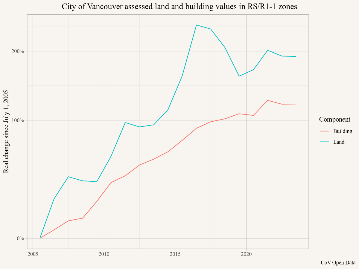
Again, the claim that building values stayed the same has no basis in reality. Readers interested in more detail are encouraged to use individual property data and match individual lots over time to further refine these estimates.