2 R, RStudio, and the tidyverse

Statistics Canada produces a lot of high quality demographic and economic data for Canada. CMHC complements this with housing data, and municipalities across Canada often provide relevant data through their Open Data portals.

2.1 R and RStudio

We will be working in R and the RStudio IDE, although using a different editor like Visual Studio Code works just as well, especially if you are already familiar with it. Within R we will be operating within the tidyverse framework, a group of R packages that work well together and allow for intuitive operations on data via pipes.

While an introduction to R is part of the goal of this book, an we will slowly build up skills as we go, we not give a systematic introduction but rather build up skills slowly as we work on concrete examples. It may be beneficial to supplement this with a more principled introduction to R and the tidyverse.

2.2 Packages

Packages are bundled sets of functionality that expand base R. We install or upgrade packages with the install.packages`. For example, to install the tidyverse framework we type

Code

install.packages("tidyverse")

into the R console. This will install or upgrade the package and required dependencies. To make the functionality, for example the tibble function from the tibble package that is part of tidyverse, available to use we can then either access functions from the package using the :: namespace selector tibble::tibble() or first load the tibble or tidyverse package via library(tidyverse) that makes the tibble() function available without having to use the namespace selector.

Additionally, we will need a number of packages that handle data acquisition and processing for Canadian data.

Code

install.packages(c("cancensus","cansim","cmhc","tongfen"))

2.3 Basic data manipulation patterns

There are several basic data manipulation patterns that we will use throughout, and we want to give a quick overview using the Palmer Penguins dataset from the palmerpenguins package.

Code

install.packages("palmerpenguins") # install the package if needed

We will at times require additional packages like this to accomplish specialized tasks, installing packages in R is generally a simple and pain-free procedure.

Code

# install.packages("palmerpenguins") # install the package if needed
library(palmerpenguins)

Now we have all the functionality of the palmerpenguins package available.

2.3.1 Exploring the data

With the palmerpenguins package comes the penguins dataset, we can expect the first few rows using the head() function which displays the first few rows.

Code

head(penguins)

# A tibble: 6 × 8
  species island    bill_length_mm bill_depth_mm flipper_l…¹ body_…² sex    year
  <fct>   <fct>              <dbl>         <dbl>       <int>   <int> <fct> <int>
1 Adelie  Torgersen           39.1          18.7         181    3750 male   2007
2 Adelie  Torgersen           39.5          17.4         186    3800 fema…  2007
3 Adelie  Torgersen           40.3          18           195    3250 fema…  2007
4 Adelie  Torgersen           NA            NA            NA      NA <NA>   2007
5 Adelie  Torgersen           36.7          19.3         193    3450 fema…  2007
6 Adelie  Torgersen           39.3          20.6         190    3650 male   2007
# … with abbreviated variable names ¹flipper_length_mm, ²body_mass_g

The str() function offers another convenient way to get an overview over the data.

Code

str(penguins)

tibble [344 × 8] (S3: tbl_df/tbl/data.frame)
 $ species          : Factor w/ 3 levels "Adelie","Chinstrap",..: 1 1 1 1 1 1 1 1 1 1 ...
 $ island           : Factor w/ 3 levels "Biscoe","Dream",..: 3 3 3 3 3 3 3 3 3 3 ...
 $ bill_length_mm   : num [1:344] 39.1 39.5 40.3 NA 36.7 39.3 38.9 39.2 34.1 42 ...
 $ bill_depth_mm    : num [1:344] 18.7 17.4 18 NA 19.3 20.6 17.8 19.6 18.1 20.2 ...
 $ flipper_length_mm: int [1:344] 181 186 195 NA 193 190 181 195 193 190 ...
 $ body_mass_g      : int [1:344] 3750 3800 3250 NA 3450 3650 3625 4675 3475 4250 ...
 $ sex              : Factor w/ 2 levels "female","male": 2 1 1 NA 1 2 1 2 NA NA ...
 $ year             : int [1:344] 2007 2007 2007 2007 2007 2007 2007 2007 2007 2007 ...

We can also type View(penguins) into the console to view the dataset in a spreadsheet form.

2.3.2 Basic data manipulation

To manipulate and visualize the data we load the tidyverse package.

Code

library(tidyverse)

We will explore some common data manipulation and visualization workflows.

2.3.2.1 Count groups

To see how many rows there are for each species we ‘pipe’ the penguins dataset into the count() verb. Pipes are how we can stepwise transform data, the pipe operator is given by %>% within the tidyverse framework and now also available natively in base R via |>. These two function (almost) the same way, and we will use both in this book.

Code

penguins |> count(species)

# A tibble: 3 × 2
  species       n
  <fct>     <int>
1 Adelie      152
2 Chinstrap    68
3 Gentoo      124

This gives us the count of each species in the dataset, the pipe |> inserts the left hand side as the first argument in the count() function. We could have equivalently written this without the pipe operator as count(penguins,species).

2.3.2.2 Group and summarize

The usefulness of the pipe operator becomes clear when we chain several data transformations. If we want to know the mean bill length by species, we group by species and summarize the data.

Code

penguins |> 
  group_by(species) |>
  summarize(bill_length_mm=mean(bill_length_mm, na.rm=TRUE))

# A tibble: 3 × 2
  species   bill_length_mm
  <fct>              <dbl>
1 Adelie              38.8
2 Chinstrap           48.8
3 Gentoo              47.5

Here we explicitly specify how missing values should be treated when summarizing, na.rm=TRUE says that NA values should be ignored when computing the mean.

2.3.3 Visualizing data

We can visualize the data using ggplot. For this we have to specify the mapping aesthetics, we plot the bill length on the x-axis, the depth on the y-axis, colour by species and plot the data as points. The labs() function allows us to customize the graph labels.

Code

ggplot(penguins,aes(x=bill_length_mm,y=bill_depth_mm,colour=species)) +
  geom_point() +
  labs(title="Penguin bill length vs depth",
       x="Bill length  (mm)",y="Bill depth (mm)",
       colour="Penguin species",
       caption="Palmer Station Antarctica LTER")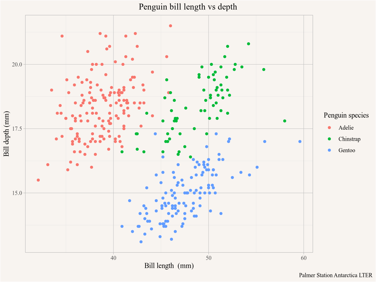

2.3.3.1 Add regression lines

As an aside we note the Simpson’s paradox, in the overall dataset the bill depth declines with length, but if we look separately within each species the bill depth increases with bill length. To make that explicit we can add regression lines using the geom_smooth function using lm (linear model) as the smoothing method.

Code

ggplot(penguins,aes(x=bill_length_mm,y=bill_depth_mm,colour=species)) +
  geom_point() +
  geom_smooth(method="lm") +
  geom_smooth(method="lm", colour="black") +
  labs(title="Penguin bill length vs depth",
       x="Bill length  (mm)",y="Bill depth (mm)",
       colour="Penguin species",
       caption="Palmer Station Antarctica LTER")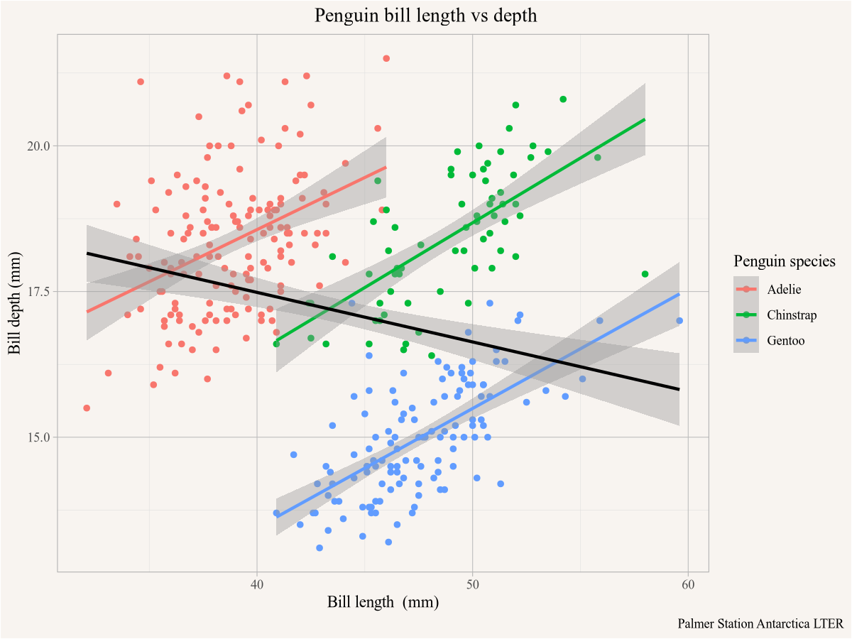

The first geom_smooth() function will add a regression line for each species, distinguished by colour in the plot aesthetics. Overriding the colour argument in the second geom_smooth() function will forget that the data was coloured by species and add the black regression line run on the entire dataset.

2.3.4 More data manipulations

There are several common data manipulation steps that we will employ frequently.

2.3.4.1 Filtering rows

Often we are only interested in subsets of the data, we can filter the rows in the dataset by using the filter verb from the dplyr package that is part of tidyverse. For example, if we want to take the previous plot but only show it for penguins on the island of Biscoe we can filter the data accordingly before plotting it.

Code

penguins |>
  filter(island=="Biscoe") |>
ggplot(aes(x=bill_length_mm,y=bill_depth_mm,colour=species)) +
  geom_point() +
  geom_smooth(method="lm") +
  geom_smooth(method="lm", colour="black") +
  labs(title="Penguin bill length vs depth",
       subtitle="Biscoe island only",
       x="Bill length  (mm)",y="Bill depth (mm)",
       colour="Penguin species",
       caption="Palmer Station Antarctica LTER")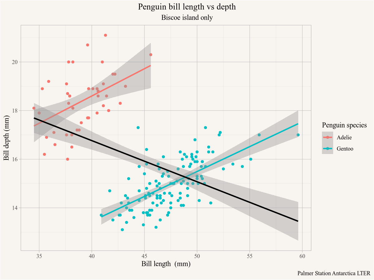

2.3.4.2 Selecting columns

Instead of filtering rows it can be useful to select a subset of the columns to remove columns we don’t need and de-clutter the dataset. This is especially useful when producing tables. If we want a table of the numeric data fields of all female Adelie penguins on the island of Biscoe observed in 2007 we can filter by sex and island and select the columns we want.

Code

penguins |>
  filter(island=="Biscoe", sex=="female", species=="Adelie", year==2007) |>
  select(where(is.numeric),-year)

# A tibble: 5 × 4
  bill_length_mm bill_depth_mm flipper_length_mm body_mass_g
           <dbl>         <dbl>             <int>       <int>
1           37.8          18.3               174        3400
2           35.9          19.2               189        3800
3           35.3          18.9               187        3800
4           40.5          17.9               187        3200
5           37.9          18.6               172        3150

2.3.4.3 Mutating data

We often want to change data fields, or compute new columns from existing ones. For example, if we want to convert the body mass from g to kg we can add a new column using mutate for that.

Code

penguin_selection <- penguins |>
  filter(island=="Biscoe", sex=="female", species=="Adelie", year==2007) |>
  mutate(body_mass_kg=body_mass_g/1000) |>
  select(where(is.numeric),-year,-body_mass_g)

penguin_selection

# A tibble: 5 × 4
  bill_length_mm bill_depth_mm flipper_length_mm body_mass_kg
           <dbl>         <dbl>             <int>        <dbl>
1           37.8          18.3               174         3.4 
2           35.9          19.2               189         3.8 
3           35.3          18.9               187         3.8 
4           40.5          17.9               187         3.2 
5           37.9          18.6               172         3.15

2.3.4.4 Pivoting data

The data in our penguin_selection dataset above is in wide form, all the different variables are in their own column. Often it is useful to convert it to long form, where we only have one value column with the numeric values and another column specifying the type of measurement. In this case it is useful to add an identification column so that we know which measurements belong to the same penguin. We can just label the penguins by row number.

Code

penguin_selection_long <- penguin_selection |>
  mutate(ID=row_number()) |>
  pivot_longer(-ID,names_to="Metric",values_to="Value")

penguin_selection_long |> head()

# A tibble: 6 × 3
     ID Metric            Value
  <int> <chr>             <dbl>
1     1 bill_length_mm     37.8
2     1 bill_depth_mm      18.3
3     1 flipper_length_mm 174  
4     1 body_mass_kg        3.4
5     2 bill_length_mm     35.9
6     2 bill_depth_mm      19.2

We can do the reverse transformation, going from long form to wide form, using pivot_wider.

Code

penguin_selection_long |>
  pivot_wider(names_from = Metric,values_from = Value)

# A tibble: 5 × 5
     ID bill_length_mm bill_depth_mm flipper_length_mm body_mass_kg
  <int>          <dbl>         <dbl>             <dbl>        <dbl>
1     1           37.8          18.3               174         3.4 
2     2           35.9          19.2               189         3.8 
3     3           35.3          18.9               187         3.8 
4     4           40.5          17.9               187         3.2 
5     5           37.9          18.6               172         3.15

This recovers the previous form of the data, with the added ID column.

2.4 Canadian data packages

During the course of this book we will make heavy use of several R packages to facilitate data access to Canadian data, we will introduce them in this chapter.