library(canpumf)
#> canpumf.cache_path is not set.
#> Downloaded data is stored in tempdir() and discarded when this R session ends, so it will be re-downloaded next time.
#> To persist data across sessions, set a cache directory:
#>   options(canpumf.cache_path = "~/canpumf_cache")
#> Add that line to your .Rprofile to make it permanent.
library(dplyr)
#>
#> Attaching package: 'dplyr'
#> The following objects are masked from 'package:stats':
#>
#>     filter, lag
#> The following objects are masked from 'package:base':
#>
#>     intersect, setdiff, setequal, union
library(ggplot2)
options(canpumf.cache_path = Sys.getenv("COMPILE_VIG_CANPUMF"))
The package supports Census PUMF from 1971 through 2021, covering
individuals, hierarchical, households, and families variants depending
on the year. The 2021 and 2016 files are available via direct download;
older years must be ordered through Statistics Canada’s EFT portal and
placed in the directory pointed to by the
canpumf.cache_path option.
census_2021 <- get_pumf("Census",version="2021") As a simple application we look at household maintainer rates by age group for select metro areas, using standard weights.
census_2021 |>
  filter(CMA %in% c("Vancouver","Toronto","Montréal","Québec")) |>
  filter(PRIHM!="Not applicable") |>
  filter(AGEGRP!="Not available") |>
  summarise(across(matches("WEIGHT|WT\\d+"),sum),
            .by=c(CMA,AGEGRP,PRIHM)) |>
  mutate(Share=WEIGHT/sum(WEIGHT),.by=c(CMA,AGEGRP)) |>
  filter(PRIHM=="Person is primary maintainer") |>
  ggplot(aes(y=AGEGRP,x=Share,fill=CMA)) +
  geom_bar(stat="identity",position="dodge") +
  scale_x_continuous(labels=scales::percent) +
  labs(title="Age-specifc household maintainer rates",
       y="Age group",
       x="Household maintainer rate",
       caption="StatCan Census 2021 PUMF")
#> Warning: Missing values are always removed in SQL aggregation functions.
#> Use `na.rm = TRUE` to silence this warning
#> This warning is displayed once every 8 hours.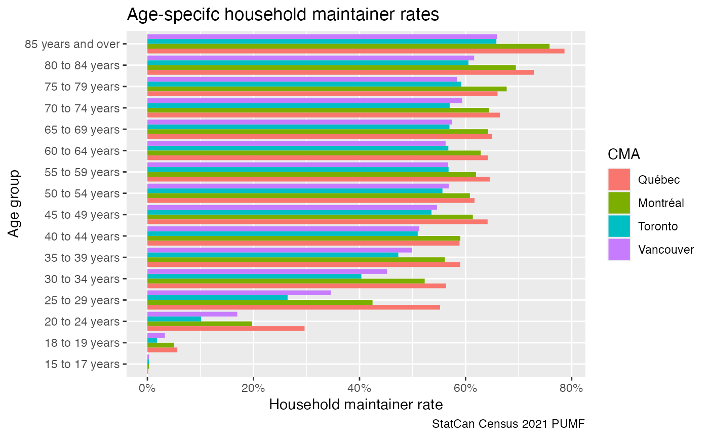
Census PUMF data is quite rich and fairly accurate when slicing it coarsely like this, but it’s always good to check for variability in the data. Census PUMF (for the recent years) comes with 16 replication weights, and we can look at the range they provide for the estimates.
census_2021 |>
  filter(CMA %in% c("Vancouver","Toronto","Montréal","Québec")) |>
  filter(PRIHM!="Not applicable") |>
  filter(AGEGRP!="Not available") |>
  summarise(across(matches("WEIGHT|WT\\d+"),sum),
            .by=c(CMA,AGEGRP,PRIHM)) |>
  collect() |>
  tidyr::pivot_longer(matches("WT\\d+"),names_to="Weights") |>
  mutate(Share=WEIGHT/sum(WEIGHT),
         Share_bsw=value/sum(value),
         .by=c(CMA,AGEGRP,Weights)) |>
  filter(PRIHM=="Person is primary maintainer") |>
  ggplot(aes(y=AGEGRP,fill=CMA)) +
  geom_bar(aes(x=Share),stat="identity",position="dodge") +
  geom_boxplot(aes(x=Share_bsw, group=interaction(CMA,AGEGRP)), fill=NA,shape=1, position="dodge") +
  scale_x_continuous(labels=scales::percent) +
  labs(title="Age-specifc household maintainer rates",
       y="Age group",
       x="Household maintainer rate (and replication weight ranges)",
caption="StatCan Census 2021 PUMF") 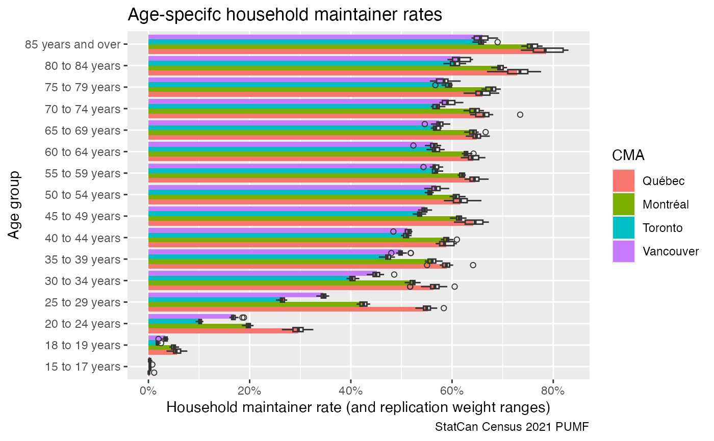
However, if we want a deeper understanding of the robustness of the
results we can add bootstrap weights, by default
add_bootstrap_weights will add 500 bootstrap weights and
save them to the database for later reference.
census_2021 |>
  filter(CMA %in% c("Vancouver","Toronto","Montréal","Québec")) |>
  filter(PRIHM!="Not applicable") |>
  filter(AGEGRP!="Not available") |>
  add_bootstrap_weights("WEIGHT") |>
  summarise(across(matches("WEIGHT|WT\\d+|CPBSW\\d+"),sum),
            .by=c(CMA,AGEGRP,PRIHM)) |>
  collect() |>
  tidyr::pivot_longer(matches("CPBSW\\d+"),names_to="Weights") |>
  mutate(Share=WEIGHT/sum(WEIGHT),
         Share_bsw=value/sum(value),
         .by=c(CMA,AGEGRP,Weights)) |>
  filter(PRIHM=="Person is primary maintainer") |>
  ggplot(aes(y=AGEGRP,fill=CMA)) +
  geom_bar(aes(x=Share),stat="identity",position="dodge") +
  geom_boxplot(aes(x=Share_bsw, group=interaction(CMA,AGEGRP)), fill=NA,shape=1, position="dodge") +
  scale_x_continuous(labels=scales::percent) +
  labs(title="Age-specifc household maintainer rates",
       y="Age group",
       x="Household maintainer rate (and bootstrap weight ranges)",
caption="StatCan Census 2021 PUMF") 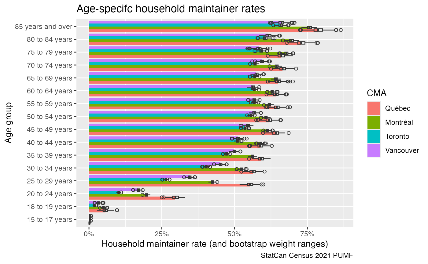
census_2021 |> close_pumf()