library(dplyr)
#>
#> Attaching package: 'dplyr'
#> The following objects are masked from 'package:stats':
#>
#>     filter, lag
#> The following objects are masked from 'package:base':
#>
#>     intersect, setdiff, setequal, union
library(tidyr)
library(ggplot2)
library(canpumf)
#> canpumf.cache_path is not set.
#> Downloaded data is stored in tempdir() and discarded when this R session ends, so it will be re-downloaded next time.
#> To persist data across sessions, set a cache directory:
#>   options(canpumf.cache_path = "~/canpumf_cache")
#> Add that line to your .Rprofile to make it permanent.
options(canpumf.cache_path = Sys.getenv("COMPILE_VIG_CANPUMF"))
The LFS is one of the most-used PUMF series, since January 2021 the LFS PUMF is now easily available for direct download instead of needing to request it via EFT. This makes it very easy to integrate the LFS into reproducible workflows.
The canpumf package has two functions to facilitate
access to the LFS PUMF. The first lists all LFS pumf versions that are
available for direct download.
list_canpumf_collection() |>
  filter(Acronym=="LFS")
#> # A tibble: 90 × 5
#>    Title               Acronym Version `Survey Number` url
#>    <chr>               <chr>   <chr>   <chr>           <chr>
#>  1 Labour Force Survey LFS     2026-05 3701            https://www150.statcan.g…
#>  2 Labour Force Survey LFS     2026-04 3701            https://www150.statcan.g…
#>  3 Labour Force Survey LFS     2026-03 3701            https://www150.statcan.g…
#>  4 Labour Force Survey LFS     2026-02 3701            https://www150.statcan.g…
#>  5 Labour Force Survey LFS     2026-01 3701            https://www150.statcan.g…
#>  6 Labour Force Survey LFS     2025    3701            https://www150.statcan.g…
#>  7 Labour Force Survey LFS     2024    3701            https://www150.statcan.g…
#>  8 Labour Force Survey LFS     2023    3701            https://www150.statcan.g…
#>  9 Labour Force Survey LFS     2022    3701            https://www150.statcan.g…
#> 10 Labour Force Survey LFS     2021    3701            https://www150.statcan.g…
#> # ℹ 80 more rows
The second one fetches and loads the LFS data. For example, to download the LFS pumf for 2022 we use
lfs_2022 <- get_pumf("LFS","2022")

lfs_2022 |>
  select(1:5) |>
  head(10)
#> # A query:  ?? x 5
#> # Database: DuckDB 1.5.4 [root@Darwin 25.5.0:R 4.6.0//Users/jens/data/pumf.data/LFS/LFS.duckdb]
#>    REC_NUM SURVYEAR SURVMNTH LFSSTAT                    PROV
#>      <int>    <int>    <int> <fct>                      <fct>
#>  1       1     2022        1 Not in labour force        Quebec
#>  2       2     2022        1 Employed, at work          British Columbia
#>  3       3     2022        1 Employed, at work          British Columbia
#>  4       4     2022        1 Employed, at work          Nova Scotia
#>  5       5     2022        1 Not in labour force        British Columbia
#>  6       6     2022        1 Unemployed                 Manitoba
#>  7       7     2022        1 Not in labour force        Manitoba
#>  8       8     2022        1 Employed, at work          Alberta
#>  9       9     2022        1 Employed, absent from work Ontario
#> 10      10     2022        1 Employed, at work          Quebec
By default the data is stored in the temporary session path,
generally we want to make sure that the canpumf.cache_path
option is set to a path to permanently cache the data.
Values come labelled, but columns are not. People working regularly
with the LFS data will likely want to keep the short default column
names, they can be converted to human readable column labels using
label_pumf_columns function.
lfs_2022 <- lfs_2022 |> label_pumf_columns()With this we can do some simple descriptive analysis. We could use
the add_bootstrap_weights function to add bootstrap weights
if desired. We focus in on February 2022 and add bootstrap weights. By
default this adds 500 weights, this will take time to generate for the
full LFS sample. For LFS data the bootstrap weight generation will
automatically stratify the generation by year and month. Here we
shortcut this by only generating bootstrap weights for the February 2022
data after calling collect, so they just get generated in memory for the
resulting tibble.
lfs_2022_02_data <- lfs_2022 |>
  filter(`Survey month`==2) |>
  collect() |>
  add_bootstrap_weights(weight_col = "Standard final weight", seed = 42)
#>   Replicate 50 / 500 ...
#>   Replicate 100 / 500 ...
#>   Replicate 150 / 500 ...
#>   Replicate 200 / 500 ...
#>   Replicate 250 / 500 ...
#>   Replicate 300 / 500 ...
#>   Replicate 350 / 500 ...
#>   Replicate 400 / 500 ...
#>   Replicate 450 / 500 ...
#>   Replicate 500 / 500 ...
For this vignette we look at gender-specific labour force status statistics for the 20 to 64 year old population, computing age-adjusted rates to even out age-specific effects.
data <- lfs_2022_02_data |>
  filter(substr(`Five-year age group of respondent`,0,2) %in% seq(20,60,5)) |>
  filter(`Labour force status`!="Not in labour force") |>
  summarise(across(matches("Standard final weight|CPBSW\\d+"),sum),
            .by=c(`Labour force status`,`Five-year age group of respondent`,`Gender of respondent`,
                  `Marital status of respondent`)) |>
  pivot_longer(matches("Standard final weight|CPBSW\\d+"),names_to="Weight",values_to="Count") |>
  group_by(`Five-year age group of respondent`,`Gender of respondent`,
           `Marital status of respondent`, Weight) |>
  mutate(Share=ifelse(Count==0,0,Count/sum(Count))) |>
  ungroup()

data_age_adjusted <- data %>%
  left_join((.) |>
              summarize(Count=sum(Count),
                        .by=c(`Five-year age group of respondent`,`Gender of respondent`,Weight)) |>
              mutate(P_age__gender=Count/sum(Count),
                     .by=c(`Gender of respondent`,Weight)) |>
              select(`Gender of respondent`,`Five-year age group of respondent`,Weight,P_age__gender),
            by=c("Gender of respondent","Five-year age group of respondent","Weight")) |>
  summarise(age_adjusted=sum(Share*P_age__gender),
            .by=c(`Gender of respondent`,`Labour force status`,`Marital status of respondent`, Weight))

data_age_adjusted |>
  filter(`Labour force status`=="Unemployed") |>
  ggplot(aes(x=age_adjusted, y=`Marital status of respondent`, fill=`Gender of respondent`)) +
  geom_boxplot() +
  geom_point(shape=21,data=~filter(.,Weight=="Standard final weight"),position=position_dodge(width=0.75)) +
  scale_x_continuous(labels=scales::percent) +
  labs(title="Unemployment rates of 20 to 64 year olds in February 2022",
       x="Age-adjusted unemployment rate",
       caption="StatCan LFS PUMF 2022-02")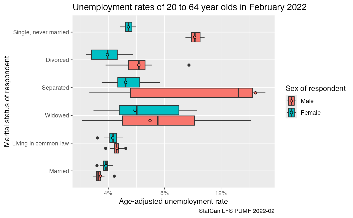
We can similarly compute the age-adjusted participation rate by gender and marital status.
data2 <- lfs_2022_02_data |>
  filter(substr(`Five-year age group of respondent`,0,2) %in% seq(20,60,5)) |>
  summarise(across(matches("Standard final weight|CPBSW\\d+"),sum),
            .by=c(`Labour force status`, `Five-year age group of respondent`,
                  `Gender of respondent`, `Marital status of respondent`)) |>
  pivot_longer(matches("Standard final weight|CPBSW\\d+"),names_to="Weight",values_to="Count") |>
  mutate(Share=ifelse(Count==0,0,Count/sum(Count)),
         .by=c(`Five-year age group of respondent`,`Gender of respondent`,
               `Marital status of respondent`, Weight))

data_age_adjusted2 <- data2 %>%
  left_join((.) |>
              summarize(Count=sum(Count),
                        .by=c(`Five-year age group of respondent`,`Gender of respondent`,Weight)) |>
              mutate(P_age__sex=Count/sum(Count),
                     .by=c(`Gender of respondent`,Weight)) |>
              select(`Gender of respondent`,`Five-year age group of respondent`,Weight,P_age__sex),
            by=c("Gender of respondent","Five-year age group of respondent","Weight")) |>
  summarise(age_adjusted=sum(Share*P_age__sex),
            .by=c(`Gender of respondent`,`Labour force status`,`Marital status of respondent`, Weight))

data_age_adjusted2 |>
  filter(`Labour force status`=="Not in labour force") |>
  ggplot(aes(x=1-age_adjusted, y=`Marital status of respondent`, fill=`Gender of respondent`)) +
  geom_boxplot() +
  geom_point(shape=21,data=~filter(.,Weight=="Standard final weight"),position=position_dodge(width=0.75)) +
  scale_x_continuous(labels=scales::percent) +
  labs(title="Labour force participation rates of 20 to 64 year olds in February 2022",
       x="Age-adjusted participation rate",
       caption="StatCan LFS PUMF 2022-02")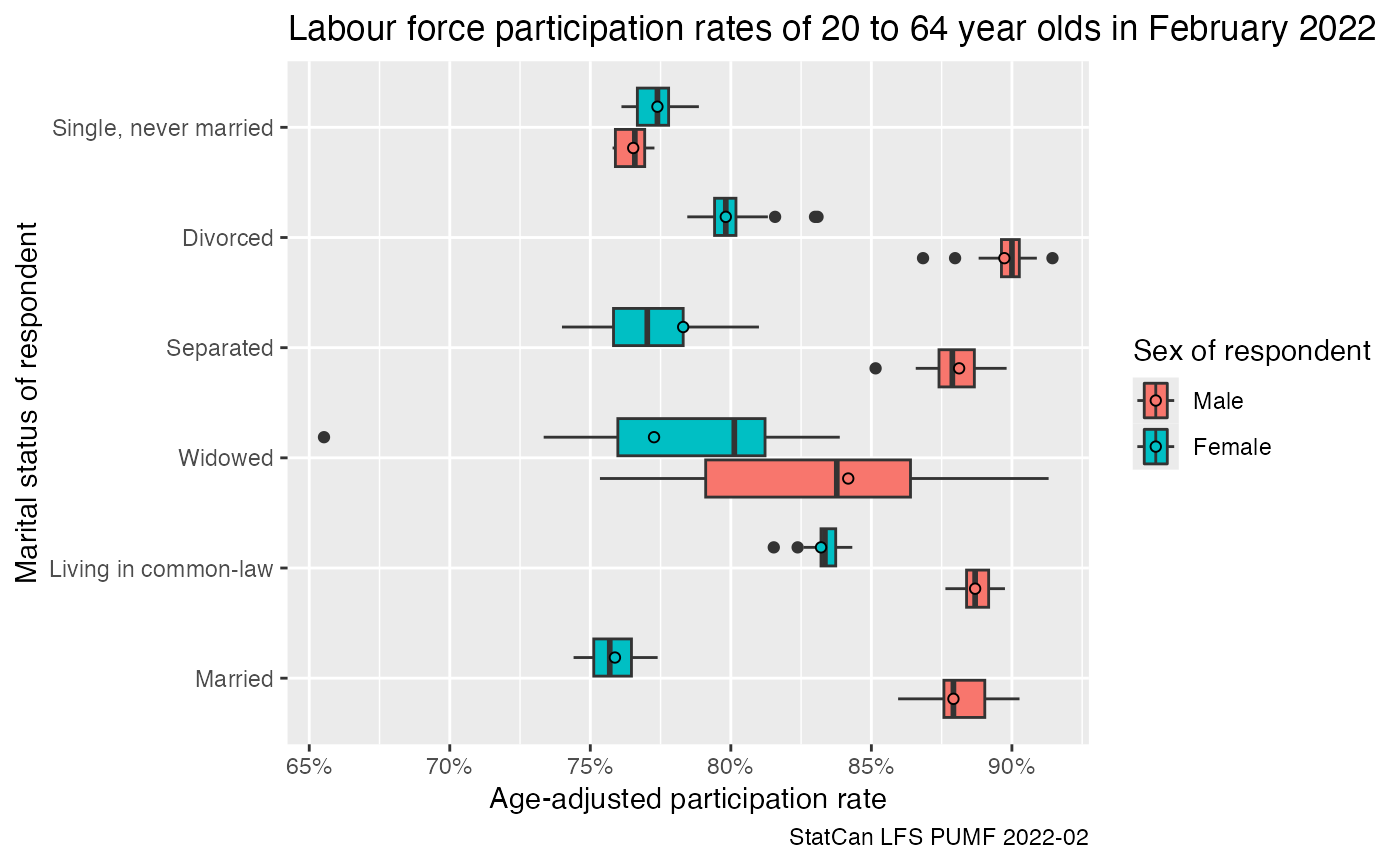
Narrowing it down a bit to only look at the share of the population employed and at work in February 2022 drops these shares a bit.
data_age_adjusted2 |>
  filter(`Labour force status`=="Employed, at work") |>
  ggplot(aes(x=age_adjusted, y=`Marital status of respondent`, fill=`Gender of respondent`)) +
  geom_boxplot() +
  geom_point(shape=21,data=~filter(.,Weight=="Standard final weight"),position=position_dodge(width=0.75)) +
  scale_x_continuous(labels=scales::percent) +
  labs(title="Share of 20 to 64 year olds working in February 2022",
       x="Age-adjusted share at work",
       caption="StatCan LFS PUMF 2022-02")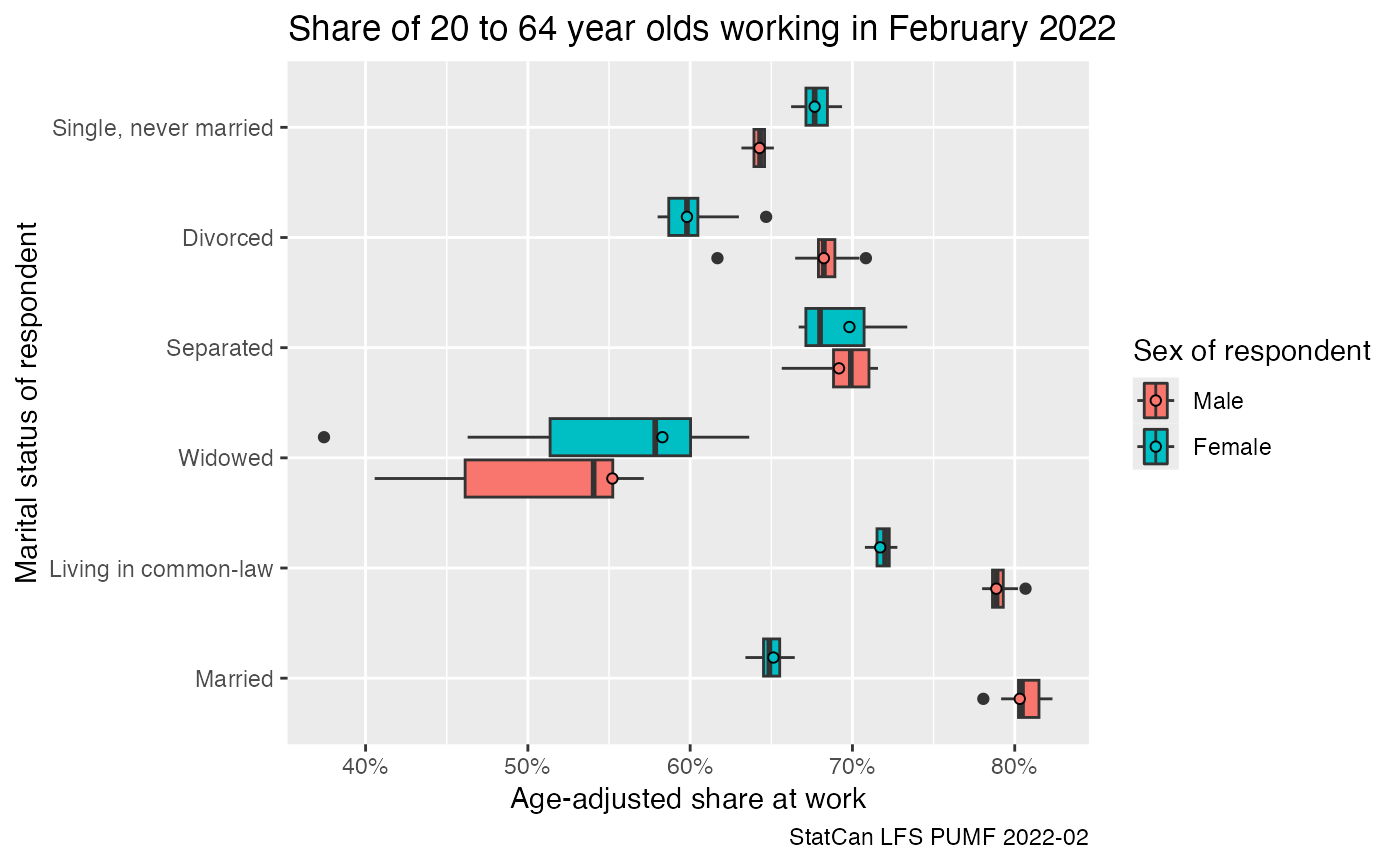
It’s good practice to close the database connection after being done with a specific task.
lfs_2022 |> close_pumf()Derived connections, like the one to the February 2022 table, will automatically be closed too.
Timelines
LFS data can also easily be accessed across time.
lfs_pumf <- get_pumf("LFS", refresh="auto")We can now easily extract time series data, we want to perform as
many operations as possible at the database level. There are several
convenience functions when working with the LFS data, one is
add_lfs_SURVDATE which adds a SURVDATE column
based on the survey year and month.
unemployment_stats <- lfs_pumf |>
  filter(LFSSTAT !="Not in labour force") |>
  filter(AGE_12 %in% c("25 to 29 years","30 to 34 years", "35 to 39 years")) |>
  mutate(jd=case_when(is.na(DURJLESS) ~ "Not applicable",
                      DURJLESS<12 ~ "Less than one year",
                      TRUE ~ "One year or more")) |>
  add_lfs_SURVDATE() |>
  summarize(Count=sum(FINALWT),.by=c(SURVDATE,jd,AGE_12)) |>
  mutate(Share=Count/sum(Count),.by=c(SURVDATE,AGE_12)) |>
  filter(jd!="Not applicable")


unemployment_stats |>
  ggplot(aes(x=SURVDATE,y=Share,colour=AGE_12)) +
  geom_line() +
  facet_wrap(~jd) +
  scale_y_continuous(labels=scales::percent_format()) +
  labs(title="Unemployment by duration of unemployment",
       y="Unemployment rate",x=NULL,
       colour="Age group",
       caption="StatCan LFS (PUMF)")
#> Warning: Missing values are always removed in SQL aggregation functions.
#> Use `na.rm = TRUE` to silence this warning
#> This warning is displayed once every 8 hours.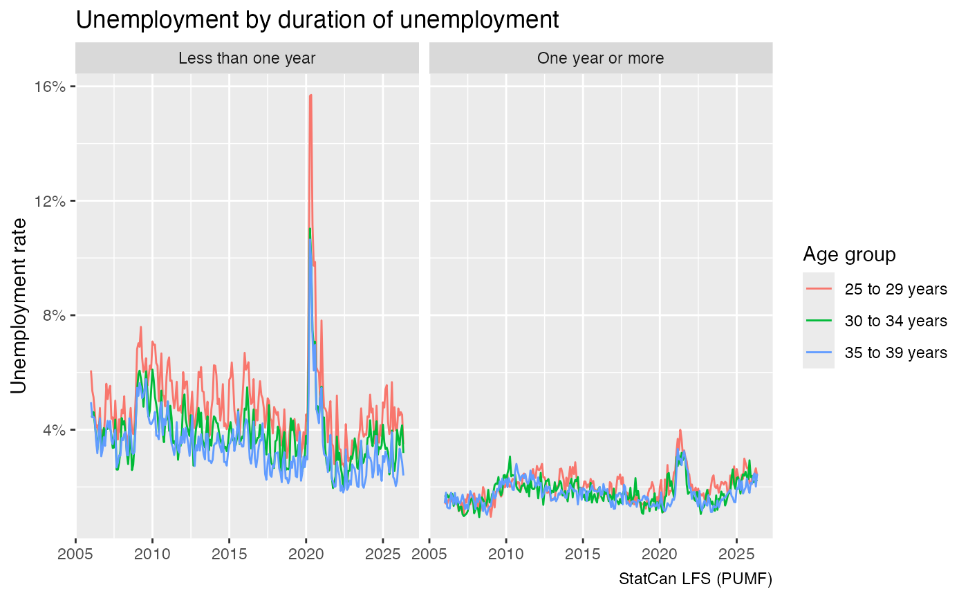
Before plotting we could call collect, but this does not
need to be done explicitly.
Because the data is efficiently organised in DuckDB, this query runs quite fast despite no explicit indexing of the database, taking less than half a second.
microbenchmark::microbenchmark(collect(unemployment_stats)) |>
  boxplot()
#> Warning in microbenchmark::microbenchmark(collect(unemployment_stats)): less
#> accurate nanosecond times to avoid potential integer overflows
The SEX variable has been recategorized into the GENDER concept
starting in 2011, older LFS PUMF data still uses SEX. We can harmonize
this by coalescing the values to create a new GENDER_SEX
column as done by the convenience function
add_lfs_GENDER_SEX.
lfs_pumf |>
  filter(LFSSTAT !="Not in labour force") |>
  add_lfs_SURVDATE() |>
  add_lfs_GENDER_SEX() |>
  summarise(Count=sum(FINALWT),.by=c(SURVDATE,LFSSTAT,GENDER_SEX)) |>
  mutate(Share=Count/sum(Count),.by=c(SURVDATE,GENDER_SEX)) |>
  filter(LFSSTAT=="Unemployed") |>
  ggplot(aes(x=SURVDATE,y=Share,colour=GENDER_SEX)) +
  geom_line() +
  scale_y_continuous(labels=scales::percent_format()) +
  labs(title="Unemployment sex/gender",
       y="Unemployment rate",x=NULL,
       colour="Gender",
       caption="StatCan LFS (PUMF)")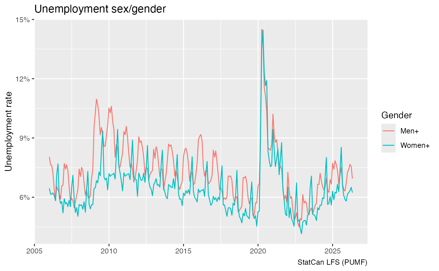
lfs_pumf |> close_pumf()