Additional datasets: Annual T1FF taxfiler data
Dataset background and example usage
Source:vignettes/Taxfiler_Data.Rmd
Taxfiler_Data.RmdBackground
Through collaboration with the Canadian Mortgage and Housing
Corporation (CMHC), CensusMapper has added and open-sourced annual
T1FF taxfiler data which provides an annual look at some basic
demographic variables. Data is available via the cancensus
package for the years 2001 through 2017. The T1FF dataset contains
information on:
- individual income
- government transfers
- family income
- family composition
- taxfilers by age groups
- taxfilers and dependents by age groups
- marital status and select other demographic variables
The data comes in varying Census geographies, depending on the year.
Retrieving any annual dataset via get_census will
automatically reference to the correct Census geography and attach the
correct spatial boundaries.
The taxfiler data is organized with consistent internal referencing. The identifier for the number of families in low income in 2017 is “v_TX2017_786” and that for all families is “v_TX2017_607”, and the ones for the other years are given by simply swapping out the year. This makes the variables selection process easy.
Example usage: constructing a multi-year series of families in low-income status
As an example we will explore a multi-year time series for families in low income. Data on low income families is available for years 2004 and later, we will start with 2006 just so that the data fits on a nice grid.
# Packages used for example
library(cancensus)
library(dplyr)
library(tidyr)
library(ggplot2)
library(sf)
To see all available T1FF datasets and their reference codes we can
use list_census_datasets().
list_census_datasets() %>%
  filter(grepl("taxfiler",description))
#> # A tibble: 19 × 6
#>    dataset description           attribution reference reference_url geo_dataset
#>    <chr>   <chr>                 <chr>       <chr>     <chr>         <chr>
#>  1 TX2000  2000 T1FF taxfiler d… StatCan 20… 72-212-X  https://www1… CA1996
#>  2 TX2001  2001 T1FF taxfiler d… StatCan 20… 72-212-X  https://www1… CA01
#>  3 TX2002  2002 T1FF taxfiler d… StatCan 20… 72-212-X  https://www1… CA01
#>  4 TX2003  2003 T1FF taxfiler d… StatCan 20… 72-212-X  https://www1… CA01
#>  5 TX2004  2004 T1FF taxfiler d… StatCan 20… 72-212-X  https://www1… CA01
#>  6 TX2005  2005 T1FF taxfiler d… StatCan 20… 72-212-X  https://www1… CA01
#>  7 TX2006  2006 T1FF taxfiler d… StatCan 20… 72-212-X  https://www1… CA06
#>  8 TX2007  2007 T1FF taxfiler d… StatCan 20… 72-212-X  https://www1… CA06
#>  9 TX2008  2008 T1FF taxfiler d… StatCan 20… 72-212-X  https://www1… CA06
#> 10 TX2009  2009 T1FF taxfiler d… StatCan 20… 72-212-X  https://www1… CA06
#> 11 TX2010  2010 T1FF taxfiler d… StatCan 20… 72-212-X  https://www1… CA06
#> 12 TX2011  2011 T1FF taxfiler d… StatCan 20… 72-212-X  https://www1… CA06
#> 13 TX2012  2012 T1FF taxfiler d… StatCan 20… 72-212-X  https://www1… CA11
#> 14 TX2013  2013 T1FF taxfiler d… StatCan 20… 72-212-X  https://www1… CA11
#> 15 TX2014  2014 T1FF taxfiler d… StatCan 20… 72-212-X  https://www1… CA11
#> 16 TX2015  2015 T1FF taxfiler d… StatCan 20… 72-212-X  https://www1… CA11
#> 17 TX2016  2016 T1FF taxfiler d… StatCan 20… 72-212-X  https://www1… CA16
#> 18 TX2017  2017 T1FF taxfiler d… StatCan 20… 72-212-X  https://www1… CA16
#> 19 TX2018  2018 T1FF taxfiler d… StatCan 20… 72-212-X  https://www1… CA16
And, as an example, available data vectors for one such T1FF dataset.
list_census_vectors('TX2017')
#> # A tibble: 818 × 7
#>    vector      type  label           units     parent_vector aggregation details
#>    <chr>       <fct> <chr>           <fct>     <chr>         <chr>       <chr>
#>  1 v_TX2017_1  Total Taxfilers - #   Number    NA            Additive    Tax da…
#>  2 v_TX2017_3  Total % 0-24          Percenta… v_TX2017_1    Average of… Tax da…
#>  3 v_TX2017_4  Total % 25-44         Percenta… v_TX2017_1    Average of… Tax da…
#>  4 v_TX2017_5  Total % 45-64         Percenta… v_TX2017_1    Average of… Tax da…
#>  5 v_TX2017_6  Total % 65+           Percenta… v_TX2017_1    Average of… Tax da…
#>  6 v_TX2017_7  Total Average - Age   Ratio     v_TX2017_1    Average of… Tax da…
#>  7 v_TX2017_8  Total % female        Percenta… v_TX2017_1    Average of… Tax da…
#>  8 v_TX2017_9  Total % married       Percenta… v_TX2017_1    Average of… Tax da…
#>  9 v_TX2017_10 Total % in appt       Percenta… v_TX2017_1    Average of… Tax da…
#> 10 v_TX2017_11 Total All persons - # Number    NA            Additive    Tax da…
#> # ℹ 808 more rows
This particular dataset has over 800 individual vectors. The vector
codes follow a regular pattern across different years, and we can use
this to quickly identify all the relevant variables of interest across
multiple datasets. We can utilized the CensusMapper graphical variable
selection interface, which can also be reached by calling
explore_census_vectors() from the R console. For this
example we are interested in low income families and note that the
internal CensusMapper vector for all families is of the form
*v_TX
While the geography varies across Census periods, the call to
get_census will automatically attach the correct geography
for each annual dataset. We pick four years to look at low income
families.
years <- c(2006,2011,2014,2018)
# Attribution for the dataset to be used in graphs
attribution <- dataset_attribution(paste0("TX",years))

plot_data <- years %>%
  lapply(function(year) {
    dataset <- paste0("TX",year)
    vectors <- c("Families"=paste0("v_",dataset,"_607"),
                 "CFLIM-AT"=paste0("v_",dataset,"_786"))

    get_census(dataset,regions=list(CMA="59933"),vectors = vectors,
                    geo_format = 'sf', level="CT", quiet = TRUE) %>%
      select(c("GeoUID",names(vectors))) %>%
      mutate(Year=year)
  }) %>%
  bind_rows() %>%
  mutate(share=`CFLIM-AT`/Families)
Here we also re-organized the data by year. All that’s left is to plot the data, one year at a time.
ggplot(plot_data,aes(fill=share)) +
  geom_sf(size=0.1,color="white") +
  facet_wrap("Year") +
  scale_fill_viridis_c(labels=scales::percent,option = "inferno",
                       trans="log",breaks = c(0.05,0.1,0.2,0.4)) +
  coord_sf(datum=NA,xlim=c(-123.4, -122.5), ylim=c(49.01, 49.4)) +
  labs(title="Share of census families in low income",fill="Share",
       caption=attribution)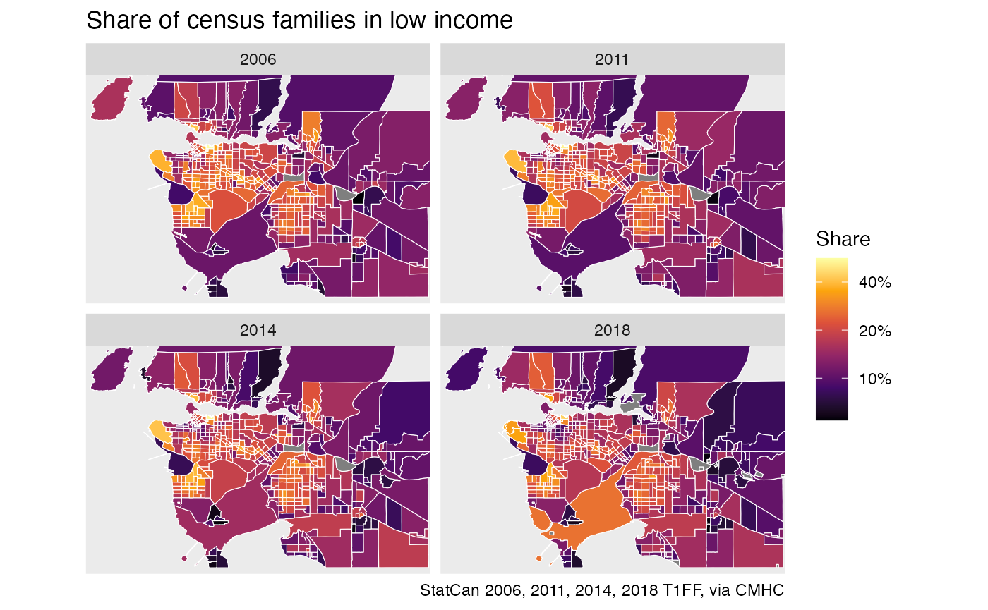
We may be tempted to re-arrange the data to create timelines, but we have to be careful as census geographies change over time. Inspecting the dataset tables at the top informs us that the 2006 through 2011 data all come on the common 2006 census geography, so the 2006 and 2011 tax data are directly comparable.
change_data <- plot_data %>%
  filter(Year==2006) %>%
  select(GeoUID,`2006`=share) %>%
  left_join(plot_data %>%
              st_set_geometry(NULL) %>%
              filter(Year==2011) %>%
              select(GeoUID,`2011`=share),
            by="GeoUID") %>%
  mutate(change=`2011`-`2006`)

ggplot(change_data,aes(fill=change)) +
  geom_sf(size=0.1) +
  scale_fill_gradient2(labels=scales::percent) +
  #scale_fill_viridis_c(labels=scales::percent,option = "inferno") +
  coord_sf(datum=NA,xlim=c(-123.4, -122.5), ylim=c(49.01, 49.4)) +
  labs(title="Change in share of census families in low income 2006-2011",fill="Percentage\npoint change",caption=dataset_attribution(paste0("TX",c(2006,2011))))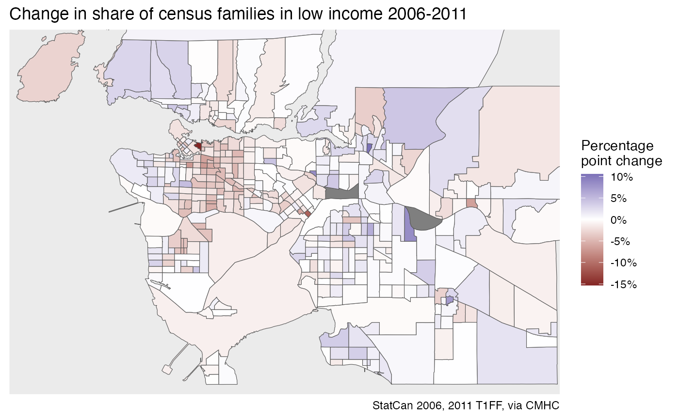
Analyzing change over longer timelines that span changes in Census geometries involves more work, the tongfen package facilitates this and provides a convenient interface for generating timelines spanning geometries from several Census years.