Finding intersecting geometries from custom data

A frequent application of census data is to evaluate values for specific areas that do not necessarily correspond to existing boundaries or administrative units. Census users may have their own defined geographies or other geospatial data of interest and want to be able to quickly and easily identify the collection of census features that correspond to that region.

The get_intersecting_geometries() function is projection agnostic and accepts any valid sf or sfc class object as input. These objects are then reprojected into lat/lon coordinates on the backend to facilitate the intersecting join on the server-side.

A simple example

As an example, suppose we are interested in understanding the housing tenure split in census tracts located near Vancouver Skytrain (rapid transit) stations. We can use the COV_SKYTRAIN_STATIONS dataset that ships with the package and is derived from the City of Vancouver Open Data portal and contains their locations. For our example we are interested in census tracts within 800m of these stations, which ships with the package.

library(cancensus)
library(dplyr)
library(ggplot2)
library(sf)

We load the example data COV_SKYTRAIN_STATIONS from the package.

cov_station_buffers <- COV_SKYTRAIN_STATIONS %>%
  st_set_crs(4326)  # needed for Ubuntu or systems with old GDAL but can otherwise be ignored

We then use the get_intersecting_geometries call to obtain the list of municipalities (CSDs) and census tracts (CTs) that intersect the 800m station buffer objects.

station_city_ids <- get_intersecting_geometries("CA16", level = "CSD", geometry = cov_station_buffers,
                                                quiet=TRUE)
station_ct_ids <- get_intersecting_geometries("CA16", level = "CT", geometry = cov_station_buffers,
                                              quiet=TRUE)

These return a list of census geographic identifiers suitable for use in the ‘region’ argument in get_census. We may be interested in the transit to work mode share in each of these buffers.

variables <- c(mode_base="v_CA16_5792",transit="v_CA16_5801",walk="v_CA16_5804")
station_city <-  get_census("CA16", regions = station_city_ids, vectors = variables, 
                            geo_format = 'sf', quiet=TRUE) %>% 
  filter(name == "Vancouver (CY)")
station_cts <-   get_census("CA16", regions = station_ct_ids, vectors = variables, 
                            geo_format = 'sf', quiet=TRUE)

To understand how these relate we plot the data.

ggplot(station_city) +
  geom_sf(fill=NA) +
  geom_sf(data=station_cts,aes(fill=((walk+transit)/mode_base))) +
  geom_sf(data=cov_station_buffers,fill=NA,alpha=0.5,color="steelblue") +
  scale_fill_viridis_c(option="magma",labels=scales::percent) +
  coord_sf(datum=NA) +
  labs(title="CTs within City of Vancouver skytrain station catchments",
       fill="Walk or\ntransit\nto work",
       caption="StatCan Census 2016")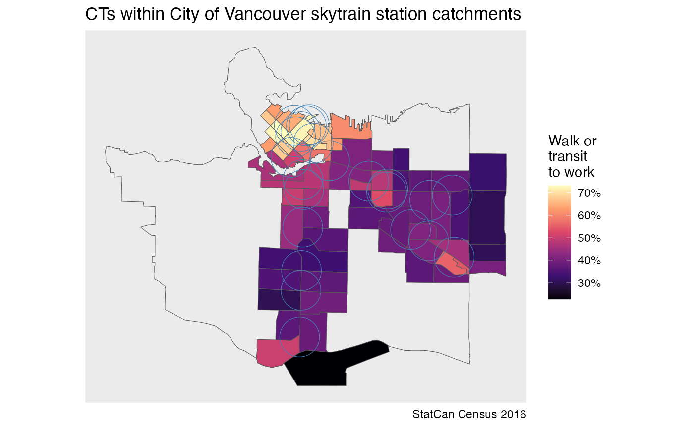

To get a closer match we can cut out the dissemination areas intersecting the station catchment areas.

station_das <-   get_intersecting_geometries("CA16", level = "DA", geometry = cov_station_buffers,
                                             quiet=TRUE) %>% 
  get_census("CA16", regions = ., vectors=variables, geo_format = 'sf', quiet=TRUE)

ggplot(station_city) +
  geom_sf(fill=NA) +
  geom_sf(data=station_das,aes(fill=((walk+transit)/mode_base))) +
  geom_sf(data=cov_station_buffers,fill=NA,alpha=0.5,color="steelblue") +
  scale_fill_viridis_c(option="magma",labels=scales::percent) +
  coord_sf(datum=NA) +
  labs(title="DAs within City of Vancouver skytrain station catchments",
       fill="Walk or\ntransit\nto work",
       caption="StatCan Census 2016")

However, API points for get_intersecting_geometries are quite limited at this point, an alternative way to obtain the same data is to first query all DAs withing the CTs identified by the previous get_intersecting_geometries call and then filter down to those intersecting the station buffers.

station_das2 <- get_census("CA16", regions = station_ct_ids, vectors=variables, 
                           geo_format = 'sf', level="DA", quiet=TRUE) %>%
  sf::st_filter(cov_station_buffers)

ggplot(station_city) +
  geom_sf(fill=NA) +
  geom_sf(data=station_das2,aes(fill=((walk+transit)/mode_base))) +
  geom_sf(data=cov_station_buffers,fill=NA,alpha=0.5,color="steelblue") +
  scale_fill_viridis_c(option="magma",labels=scales::percent) +
  coord_sf(datum=NA) +
  labs(title="DAs within City of Vancouver skytrain station catchments",
       fill="Walk or\ntransit\nto work",
       caption="StatCan Census 2016")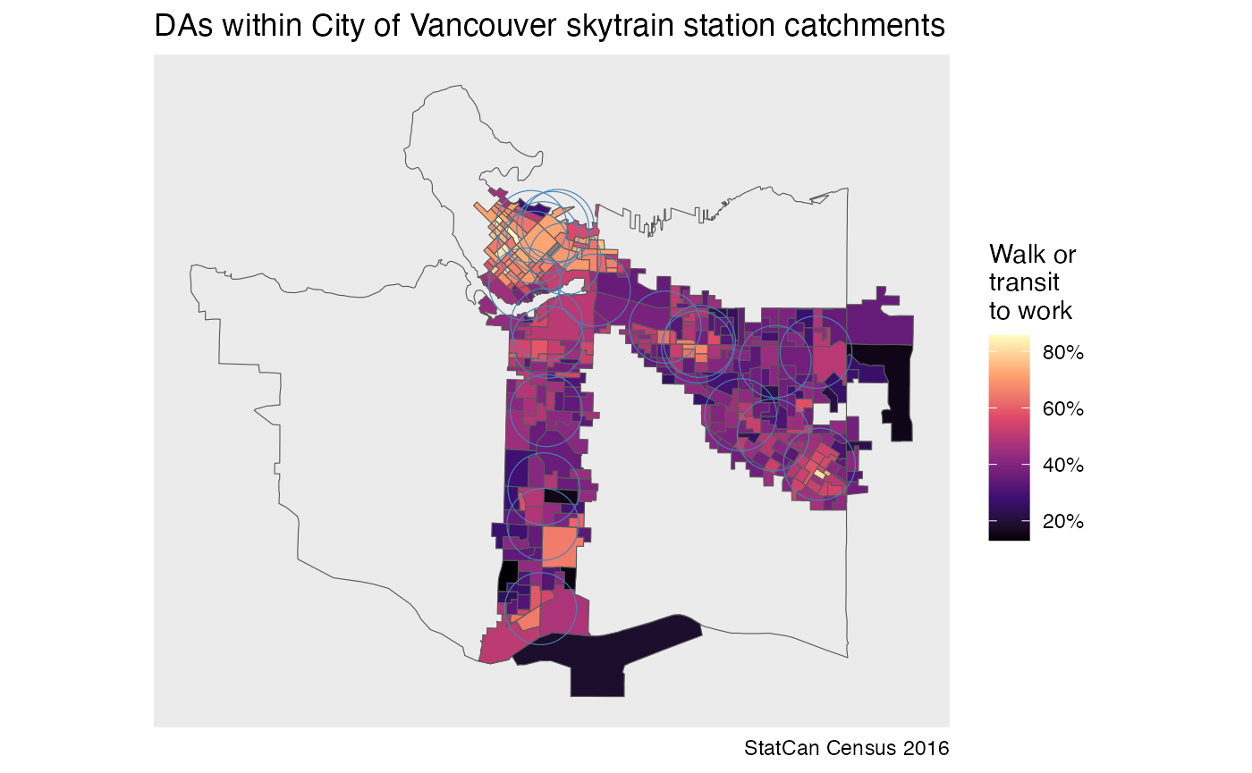

We may increase the default quotas for the get_intersecting_geometries call at some point, but while we throttling API usage and monitor server impacts of the new functionality it may be preferable to use the get_intersecting_geometries call for higher level geographies only and add a few lines of code to do the final bit of filtering in R.

Addendum

We may take this further by estimate values of census variables strictly within catchments areas. Rather than intersecting, some adjustments for spatial disaggregation and interpolation are needed. The tongfen_estimate method from the tongfen package is useful in this case. This is a related package that is designed to work in tandem with cancensus in order to facilitate census geography aggregation and is designed to make census data comparable across several censuses.

Bring custom data and identify corresponding census geographies

A simple example

Addendum